Interaction model of a farmer and a restaurant
This system describes a farm and a restaurant belonging to a same project. Consequently, they function in full cooperation.
Description of the system :
de Lapparent, A., Martin, S. & Sabatier, R. Using System Modularity to Simplify Viability Studies: An Application to a Farm-Restaurant Interaction. Environ Model Assess (2024). https://doi.org/10.1007/s10666-024-10014-w
The object computed is a viability kernel. The model is discrete in states, controls and time.
The computation takes a moment (4088s on my computer), be patient...
Model
States and controls
State variables
| Notation | Description | Number of points | Maximal value | Minimal value |
| $x_1$ | Cumulative cash flow (€) | 41 | 100 000 | 0 |
| $x_2$ | Restaurant attractivity coefficient (no unit) | 31 | 1 | 0 |
| $x_3$ | General Index for Soil Quality | 51 | 1 | 0 |
upper limit of $x_1$ can be relaxed.
Control variables
| Notation | Description | Number of points | Maximal value | Minimal value |
| $u_1$ | Choice of N-crops rotation | 126 | 126 | 1 |
| $u_2$ | Surface dedicated to market gardening (in ha) | 21 | 2 | 0.05 |
| $u_3$ | Price of a meal (in €) | 21 | 15 | 2 |
Dynamics
Overall dynamics are:
\begin{equation}
\mathcal{S}_U
\begin{cases}
x_{1}^{t+1} = x_{1}^t + G(x_{2}^t,u_{3}^t,R(x_3^t,u_1^t,u_2^t)) - E(u_{1}^t,u_{2}^t)\\
x_{2}^{t+1} = \alpha(x_{2}^t,u_{3}^t,R(x_3^t,u_1^t,u_2^t))\\
x_{3}^{t+1} = \Phi (x_{3}^t ,u_{1}^t,u_{2}^t) \\
\end{cases}
\end{equation}
with the following functions:
|
Notation |
Description |
| $R(x_3,u_1,u_2)$ | Agricultural production |
| $G(x_2,u_3,R(x_3,u_1,u_2))$ | Restaurant economic outcome |
| $\alpha(x_2,u_3,R(x_3,u_1,u_2))$ | Transition function for the restaurant attractivity |
| $\Phi(x_3,u_1,u_2)$ | Transition function for the GISQ |
| $E(u_1,u_2)$ | Cost of agricultural production |
Some dynamics require to use grid parameters. Consequently, a function has been implemented into the source file to get these values.
Constraints
There are two cconstraints in this system: the global system has to be profitable and a minimal soil quality has to be preserved in order to address sustainability concerns. These constraints take the form of thresholds on the cumulative cash flow ($x_{1} \geq x_{1min}$) and on soil quality ($x_3 \geq x_{3min}$), respectively. In other words, $(x_1^t,x_2^t,x_3^t)$ must remain in $K$ for all $t\in \mathbb{N}$ with :
\begin{equation}
K:=\{(x_1,x_2,x_3)\in \mathbb{R}^+\times [0;1]^2 \; |\; x_1\geq x_{1min} \text{ and }x_3\geq x_{3min}\}.
\label{K}
\end{equation}
Implementation parameters
Time horizon
The time horizon (for trajectory computations) is 20 years.
Algorithm parameters
Default parameters are used.
System parameters
We used the parameters for a low-hypotheses computation.
   "SYSTEM_PARAMETERS": {
       "DYNAMICS_TYPE": 2,
       "DYN_BOUND": 1,
       "DYN_BOUND_COMPUTE_METHOD": 2,
       "IS_TIMESTEP_GLOBAL": 0,
       "LIPSCHITZ_CONSTANT": 1,
       "LIPSCHITZ_CONSTANT_COMPUTE_METHOD": 2,
       "TIME_DISCRETIZATION_SCHEME": 4
   }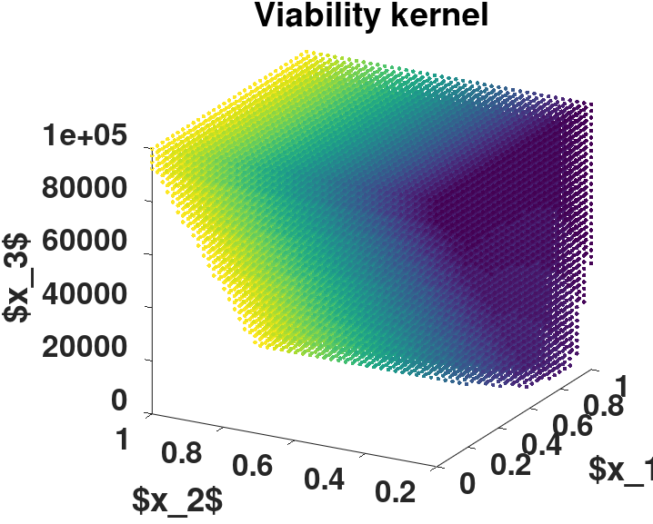
Viability kernel computed using ViabLab