This system describes a farm and a restaurant belonging to a same project. Farm production is designed to supply the restaurant, thus minimizing the need of food purchases from external suppliers. Consequently, both activities work in close cooperation, and their respective management must be carefully calibrated in order to maintain the viability of the whole project. More specifically, in the absence of other outlets, any vegetable overproduction would go unused, resulting in the loss of all corresponding production costs. An over-intensive use of the farm plots can also lead to soil depletion, thereby reducing future yields. Conversely, introducing fallow plots helps to maintain soil quality, but an underproduction of vegetables would require a purchase of additional food supply at a high price in order to meet the restaurant's needs.
This system, and the associated model, are described in the following article :
de Lapparent, A., Martin, S. & Sabatier, R. Using System Modularity to Simplify Viability Studies: An Application to a Farm-Restaurant Interaction. Environ Model Assess (2024). https://doi.org/10.1007/s10666-024-10014-w
The object computed is a viability kernel. The model is discrete in states, controls and time.
The computation takes a moment (4088s on my computer), be patient...
Model
States and controls
State variables
| Notation | Description | Number of points | Maximal value | Minimal value |
| $x_1$ | Cumulative cash flow (€) | 41 | 100 000 | 0 |
| $x_2$ | Restaurant attractivity coefficient (no unit) | 31 | 1 | 0 |
| $x_3$ | General Index for Soil Quality | 51 | 1 | 0 |
upper limit of $x_1$ can be relaxed.
Control variables
| Notation | Description | Number of points | Maximal value | Minimal value |
| $u_1$ | Choice of N-crops rotation | 126 | 126 | 1 |
| $u_2$ | Surface dedicated to market gardening (in ha) | 21 | 2 | 0.05 |
| $u_3$ | Price of a meal (in €) | 21 | 15 | 2 |
Dynamics
Overall dynamics are:
\begin{equation}
\mathcal{S}_U
\begin{cases}
x_{1}^{t+1} = x_{1}^t + G(x_{2}^t,u_{3}^t,R(x_3^t,u_1^t,u_2^t)) - E(u_{1}^t,u_{2}^t)\\
x_{2}^{t+1} = \alpha(x_{2}^t,u_{3}^t,R(x_3^t,u_1^t,u_2^t))\\
x_{3}^{t+1} = \Phi (x_{3}^t ,u_{1}^t,u_{2}^t) \\
\end{cases}
\end{equation}
with the following functions:
|
Notation |
Description |
| $R(x_3,u_1,u_2)$ | Agricultural production |
| $G(x_2,u_3,R(x_3,u_1,u_2))$ | Restaurant economic outcome |
| $\alpha(x_2,u_3,R(x_3,u_1,u_2))$ | Transition function for the restaurant attractivity |
| $\Phi(x_3,u_1,u_2)$ | Transition function for the GISQ |
| $E(u_1,u_2)$ | Cost of agricultural production |
Some dynamics require to use grid parameters. Consequently, a function has been implemented into the source file to get these values.
Constraints
There are two cconstraints in this system: the global system has to be profitable and a minimal soil quality has to be preserved in order to address sustainability concerns. These constraints take the form of thresholds on the cumulative cash flow ($x_{1} \geq x_{1min}$) and on soil quality ($x_3 \geq x_{3min}$), respectively. In other words, $(x_1^t,x_2^t,x_3^t)$ must remain in $K$ for all $t\in \mathbb{N}$ with :
\begin{equation}
K:=\{(x_1,x_2,x_3)\in \mathbb{R}^+\times [0;1]^2 \; |\; x_1\geq x_{1min} \text{ and }x_3\geq x_{3min}\}.
\end{equation}
Implementation parameters
Time horizon
The time horizon (for trajectory computations) is 20 years.
Algorithm parameters
Default parameters are used.
System parameters
We used the parameters for a low-hypotheses computation.
   "SYSTEM_PARAMETERS": {
       "DYNAMICS_TYPE": 2,
       "DYN_BOUND": 1,
       "DYN_BOUND_COMPUTE_METHOD": 2,
       "IS_TIMESTEP_GLOBAL": 0,
       "LIPSCHITZ_CONSTANT": 1,
       "LIPSCHITZ_CONSTANT_COMPUTE_METHOD": 2,
       "TIME_DISCRETIZATION_SCHEME": 4
   }
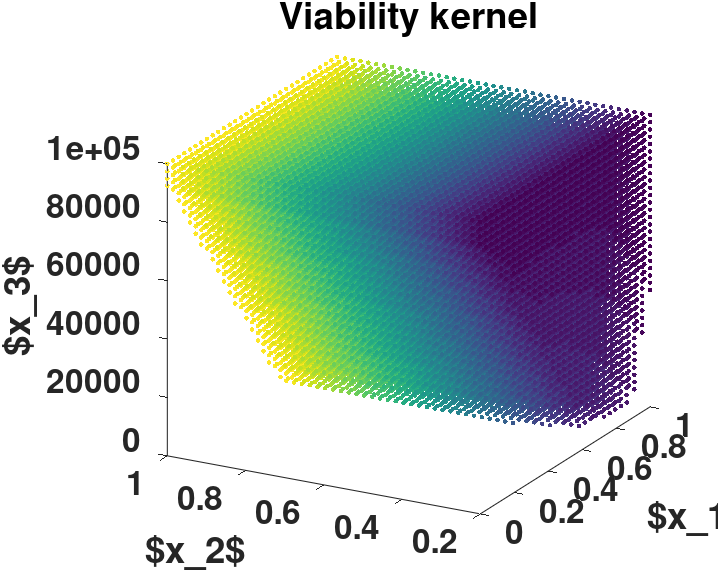
Viability kernel computed using ViabLab