Prey-predator model

Introduction

Let us consider the classic Lotka-Volterra predator-prey model with two variables: $x(t)$, the prey population size over time, and $y(t)$, the predator population size over time.
Population changes over time depend on:

• the prey reproduction rate, $\alpha$
• the prey mortality rate due to predators, $\beta$
• the predator production rate based on prey consumed, $\delta$
• the predator mortality rate, $\gamma$.

Lotka and Volterra independently proposed the following equations:

$$\left\{\begin{array}{l}x'=x(\alpha-\beta y)\\ y'=y(\delta x-\gamma)\end{array}\right.$$

Modeling a viability problem for the prey

In their article

Térence Bayen, Alain Rapaport. Minimal time crisis versus minimum time to reach a viability kernel: a case study in the prey-predator model. Optimal Control Applications and Methods, 2019, 40 (2), pp.330-350. ⟨10.1002/oca.2484⟩. ⟨hal-01943636v2⟩

the authors addressed the problem of preserving the prey population in the face of predators by keeping their numbers above a given threshold $\underline{x} > 0$ as much as possible. This amounts to ensuring that the state remains within the set

$$K(\underline{x}):=\{(x,y)\,|\, x>=\underline{x}\},$$

based on the premise that low prey density exposes the population to a risk of extinction that should be avoided as much as possible.

Using the original Lotka-Volterra equations, the authors assume constant values ​​for $\alpha=r$, $\beta=1$, and $\delta=1$. However, a control can influence predator mortality; thus, the authors set $\gamma = m + u$, where $m$ is a constant and $u$ is an excess mortality rate that can vary, with $u(t) \in [0, \bar{u}]$.

The viability problem can be summarized as follows:

\begin{equation}
\left\{
\begin{array}{l}
x'=x(r- y)\\
y'=y( x-m-u)\\
u(t) \in [0;\bar{u}]\\
\left(x(t),y(t)\right) \in K(\underline{x}):=\{(x,y)\,|\, x>=\underline{x}\}
\end{array}
\right.
\end{equation}

Solving this problem means finding the set of states $(x,y)$ from which it is possible to maintain a prey population level above $\underline{x}$ over time by manipulating prey excess mortality—in other words, the viability kernel, using the terminology of viability theory.

Results

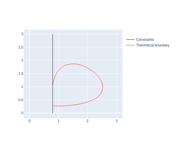
The authors provide an analytical description of this viability kernel. When $\bar{u}\geq \underline{x}-m$, by considering the invariant of this Lotka-Volterra system (which depends on $u$), $W_u(x,y):=x-(m+u)\ln x+y -r\ln y$, they construct the boundary of the viability kernel using a closed curve composed of three subsets:

• $\{(x,y) | y\geq r \text{ and }W_{\bar{u}}(x,y)=W_{\bar{u}}(\underline{x}, r) \}$.
• Let $x^+>\underline{x}$ such that $W_{\bar{u}}(x^+,r)=W_{\bar{u}}(\underline{x}, r)$,
  $\{(x,y) | y\leq r \text{ and }W_{0}(x,y)=W_{0}(x^+, r) \}$
• Let $r^-$ such that $W_{0}(\underline{x},r^-)=W_{0}(x^+, r)$,
  $\{(x,y) | x=\underline{x} \text{ and } y\in [r^-,r]\}$

The following figure shows the result for the parameters: $r=1$, $m=1$, $\bar{u}=0.5$, $\underline{x}=0.8$.

Because an analytical description of its boundary exists, this viability problem allows for testing the precision of approximations generated by generic software.

Shown below is a comparison—for $r=1$, $m=1$, $\bar{u}=0.5$, and $\underline{x}=0.8$—between the viability kernel boundary derived from its analytical description (in red) and the approximate result obtained using the ViabLab software on a regular grid of 4001×4001 points (light blue set with a dark blue boundary):

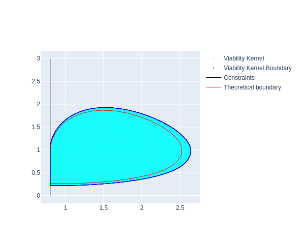
 It can be seen that the kernel approximation is well performed from the outside.