Grazing management - shoot biomass

Introduction

A major challenge in managing grazed pastures lies in reconciling conflicting objectives: increasing short-term profits while preserving the long-term viability of the rangeland. Increasing the stocking rate (number of animals per hectare) boosts short-term returns but can lead to virtually irreversible environmental degradation if the resulting grazing pressure is excessive. Conversely, maintaining an excessively low stocking rate can result in significant lost revenue.

In the article

Anderies, J., Janssen, M. & Walker, B. Grazing Management, Resilience, and the Dynamics of a Fire-driven Rangeland System. Ecosystems 5, 23–44 (2002). https://doi.org/10.1007/s10021-001-0053-9

The authors use the following model to account for the interactions between grass growth and grazing pressure:

$$
\left\{\begin{array}{ll}
c' &= r_cs-\delta_cc\\
s'&= c(a_c+r_ss)(1-\frac{s}{s^*}-\alpha_{ws}(\frac{w}{w^*})^\beta)-\gamma_gs\\
w'&=r_ww(1-\frac{w}{w^*})
\end{array}\right.
$$

Regarding the grass, $c(t)$ and $s(t)$ represent the biomass of the crown (roots plus growing points) and the shoot part, respectively, at time $t$. The parameter $s^*$ corresponds to the maximum shoot biomass per unit area, while $\gamma_g\leq 1$ represents the fraction of the shoot part removed by the grazing pressure exerted by the animals present. The crown grows at a rate $r_cs$ in the presence of shoot parts and declines at a rate $\delta_c$.
$a_c$ corresponds to the growth rate of shoot biomass per unit of crown biomass, and $r_s$ to the growth rate of shoot biomass per unit of crown biomass and per unit of shoot biomass.

Grass growth is also affected by the presence of shrubs: $w(t)$ represents shrub biomass, $r_w$ the intrinsic growth rate of shrubs, $w^*$ the maximum shrub biomass per unit area, and $w_s (=w/w^*)$ models the competitive effect of shrubs on the grass. The parameter $\beta$ measures the relative non-linearity of this effect.

The pasture manager's viability problem

The objective of rangeland management is to identify intervention strategies (adjustments to stocking rates) that reconcile two constraints: providing sufficient feed for the animals while preserving grass quality.

In the article

Martin, Sophie & Deffuant, Guillaume & Calabrese, Justin. (2011). Defining Resilience Mathematically: From Attractors To Viability. 10.1007/978-3-642-20423-4_2. 

the authors study this viability problem using a simplified grass growth model, assuming that the shrub population remains constant at its equilibrium value and that the crown biomass instantly reaches the equilibrium value associated with the shoot biomass:

$$
w = w^* \text{ and  } c = \frac{r_c}{\delta_c}s.
$$

The possible intervention on the system involves varying the grazing pressure—a variation assumed to be bounded—since purchasing or selling animals takes time :

$$
\gamma'(t) = u(t) \in [u_{min},u_{max}].
$$

The dynamics of the system are thus described by:

$$
\left\{\begin{array}{ll}
\gamma_g'&= u \in [u_{min},u_{max}]\\
s'&= \frac{r_c}{\delta_c}s(a_c+r_ss)(1-\frac{s}{s^*}-\alpha_{ws})-\gamma_gs.
\end{array}\right.
$$

The constraint regarding grass quality is modeled by a shoot biomass value falling between two limits: a lower limit to ensure regeneration and an upper limit to preserve nutritional quality. The constraint regarding livestock feed is modeled by a grazing pressure that must also remain above a certain threshold over time. The set of constraints can thus be expressed as follows:

$$
K(\underline{g},s_{min},s_{max}):=[\underline{g},1]\times [s_{min},s_{max}].
$$

Solving this problem means finding the set of states $(s, \gamma_g)$ from which it is possible to feed the herd while maintaining high-quality grass by adjusting the number of animals—in other words, the viability kernel within the framework of viability theory.

Results

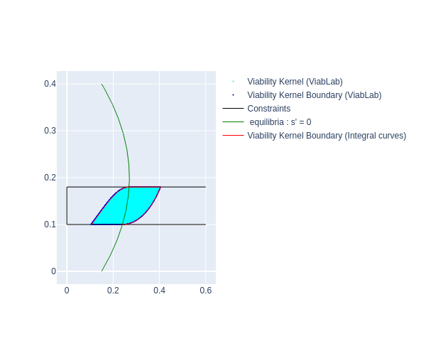
For the parameter values ​​from the article cited above ($r_c=1$, $\delta_c=1$, $a_c=0.3$, $r_s=3$, $s^*=1$, $\alpha_{ws}=0.5$, $u_{min} = -0.02$, $u_{max} = 0.02$, $\underline{g}=0$, $s_{min} = 0.1$, $s_{max} = 0.18$), the viability kernel can be obtained by calculating two integral curves (the authors of the article did not elaborate on this point).

Indeed, its boundary is defined by a closed curve formed by subsets of the boundary of the constraint set $K$ and two integral curves:

• the one originating from the point $(\gamma_g^1,s_{min}) $ with $s'(\gamma_g^1,s_{min})) = 0$ that follows the backward dynamics: 
  \begin{equation}
  \left\{\begin{array}{ll}
  \gamma_g'&= -u_{min}\\
  s'&= -(\frac{r_c}{\delta_c}s(a_c+r_ss)(1-\frac{s}{s^*}-\alpha_{ws})-\gamma_gs)\\ 
  \end{array}\right.
  \end{equation}
• the other originating from the point $(\gamma_g^2,s_{max}) $ with $s'(\gamma_g^2,s_{max})) = 0$ that follows that follows the backward dynamics: 
  \begin{equation}
  \left\{\begin{array}{ll}
  \gamma_g'&= -u_{max}\\
  s'&= -(\frac{r_c}{\delta_c}s(a_c+r_ss)(1-\frac{s}{s^*}-\alpha_{ws})-\gamma_gs)\\ 
  \end{array}\right.
  \end{equation}

The following figure shows the boundary of the viability kernel as a closed curve, along with the approximation obtained using the ViabLab software on a 2001 × 2001 grid of points. The result is consistent with the graph in the original article and is far more precise in the section of the kernel boundary that coincides with the boundary of the constraint set, as well as in the section defined by the integral curves.