Agriculture

Introduction

A major challenge in managing grazed pastures lies in reconciling conflicting objectives: increasing short-term profits while preserving the long-term viability of the rangeland. Increasing the stocking rate (number of animals per hectare) boosts short-term returns but can lead to virtually irreversible environmental degradation if the resulting grazing pressure is excessive. Conversely, maintaining an excessively low stocking rate can result in significant lost revenue.

In the article

Anderies, J., Janssen, M. & Walker, B. Grazing Management, Resilience, and the Dynamics of a Fire-driven Rangeland System. Ecosystems 5, 23–44 (2002). https://doi.org/10.1007/s10021-001-0053-9

The authors use the following model to account for the interactions between grass growth and grazing pressure:

$$
\left\{\begin{array}{ll}
c' &= r_cs-\delta_cc\\
s'&= c(a_c+r_ss)(1-\frac{s}{s^*}-\alpha_{ws}(\frac{w}{w^*})^\beta)-\gamma_gs\\
w'&=r_ww(1-\frac{w}{w^*})
\end{array}\right.
$$

Regarding the grass, $c(t)$ and $s(t)$ represent the biomass of the crown (roots plus growing points) and the shoot part, respectively, at time $t$. The parameter $s^*$ corresponds to the maximum shoot biomass per unit area, while $\gamma_g\leq 1$ represents the fraction of the shoot part removed by the grazing pressure exerted by the animals present. The crown grows at a rate $r_cs$ in the presence of shoot parts and declines at a rate $\delta_c$.
$a_c$ corresponds to the growth rate of shoot biomass per unit of crown biomass, and $r_s$ to the growth rate of shoot biomass per unit of crown biomass and per unit of shoot biomass.

Grass growth is also affected by the presence of shrubs: $w(t)$ represents shrub biomass, $r_w$ the intrinsic growth rate of shrubs, $w^*$ the maximum shrub biomass per unit area, and $w_s (=w/w^*)$ models the competitive effect of shrubs on the grass. The parameter $\beta$ measures the relative non-linearity of this effect.

The pasture manager's viability problem

The objective of rangeland management is to identify intervention strategies (adjustments to stocking rates) that reconcile two constraints: providing sufficient feed for the animals while preserving grass quality.

In the article

The authors study this viability problem using a simplified grass growth model, assuming that the maximum shoot biomass value, $s^*$, is 1 and that the impact of the shrub population is negligible—that is: 

$$
s^* = 1 \text{ et } \alpha_{ws} = 0.$$

The possible intervention on the system involves varying the grazing pressure—a variation assumed to be bounded—since purchasing or selling animals takes time :

$$
\gamma'(t) = u(t) \in [u_{min},u_{max}].
$$

The dynamics of the system are thus described by:

$$
\left\{\begin{array}{ll}
c' &= r_cs-\delta_cc\\
s'&= \frac{r_c}{\delta_c}s(a_c+r_ss)(1-s)-\gamma_gs\\
\gamma_g'&= u \in [u_{min},u_{max}]
\end{array}\right.
$$

The constraint regarding grass quality is modeled by a shoot biomass value exceeding a threshold, $s_{min}$, to ensure regrowth. The constraint regarding livestock feed is modeled by a grazing pressure that also exceeds a threshold, $\underline{g}$, over time. The set of constraints can thus be written as:

$$
K(s_{min},\underline{g}):=R^+\times [s_{min},+\infty[\times  [\underline{g},1]
$$

Solving this problem means finding the set of states $(s, \gamma_g)$ from which it is possible to feed the herd while maintaining high-quality grass by adjusting the number of animals—in other words, the viability kernel within the framework of viability theory.

Résultats

In the article cited above, the parameter values ​​are as follows: $r_c=1$, $\delta_c=1$, $a_c=0.1$,  $r_s=3$,  $s^*=1$, $u_{min} = -0.05$, $u_{max} = 0.05$, $s_{min} = 0.1$, $\underline{g}=0.65$.

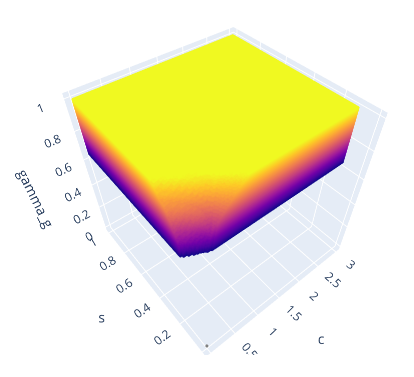
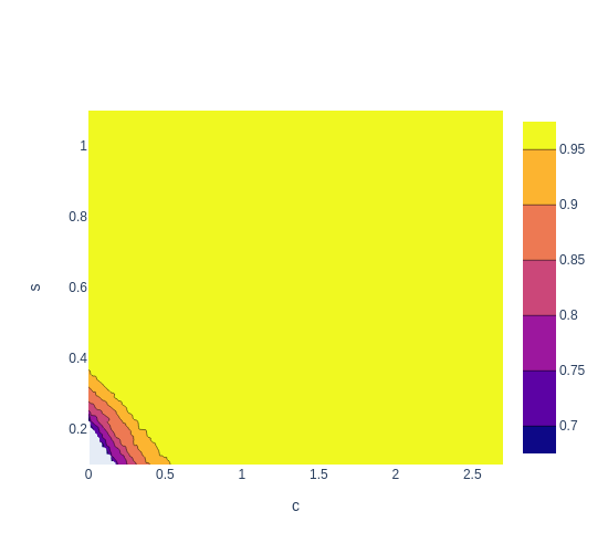
We reproduce below the approximation of the viability kernel associated with these parameter values, generated by the ViabLab software using a 201×201×201 point grid:

As expected, starting from a higher grazing pressure results in a more restricted set of shoot and crown biomass combinations for which the system is viable.

This restriction is more pronounced when the capacity to reduce this pressure is low—that is, when $u_{min}$ approaches 0.

Introduction

A major challenge in managing grazed pastures lies in reconciling conflicting objectives: increasing short-term profits while preserving the long-term viability of the rangeland. Increasing the stocking rate (number of animals per hectare) boosts short-term returns but can lead to virtually irreversible environmental degradation if the resulting grazing pressure is excessive. Conversely, maintaining an excessively low stocking rate can result in significant lost revenue.

In the article

Anderies, J., Janssen, M. & Walker, B. Grazing Management, Resilience, and the Dynamics of a Fire-driven Rangeland System. Ecosystems 5, 23–44 (2002). https://doi.org/10.1007/s10021-001-0053-9

The authors use the following model to account for the interactions between grass growth and grazing pressure:

$$
\left\{\begin{array}{ll}
c' &= r_cs-\delta_cc\\
s'&= c(a_c+r_ss)(1-\frac{s}{s^*}-\alpha_{ws}(\frac{w}{w^*})^\beta)-\gamma_gs\\
w'&=r_ww(1-\frac{w}{w^*})
\end{array}\right.
$$

Regarding the grass, $c(t)$ and $s(t)$ represent the biomass of the crown (roots plus growing points) and the shoot part, respectively, at time $t$. The parameter $s^*$ corresponds to the maximum shoot biomass per unit area, while $\gamma_g\leq 1$ represents the fraction of the shoot part removed by the grazing pressure exerted by the animals present. The crown grows at a rate $r_cs$ in the presence of shoot parts and declines at a rate $\delta_c$.
$a_c$ corresponds to the growth rate of shoot biomass per unit of crown biomass, and $r_s$ to the growth rate of shoot biomass per unit of crown biomass and per unit of shoot biomass.

Grass growth is also affected by the presence of shrubs: $w(t)$ represents shrub biomass, $r_w$ the intrinsic growth rate of shrubs, $w^*$ the maximum shrub biomass per unit area, and $w_s (=w/w^*)$ models the competitive effect of shrubs on the grass. The parameter $\beta$ measures the relative non-linearity of this effect.

The pasture manager's viability problem

The objective of rangeland management is to identify intervention strategies (adjustments to stocking rates) that reconcile two constraints: providing sufficient feed for the animals while preserving grass quality.

In the article

Martin, Sophie & Deffuant, Guillaume & Calabrese, Justin. (2011). Defining Resilience Mathematically: From Attractors To Viability. 10.1007/978-3-642-20423-4_2. 

the authors study this viability problem using a simplified grass growth model, assuming that the shrub population remains constant at its equilibrium value and that the crown biomass instantly reaches the equilibrium value associated with the shoot biomass:

$$
w = w^* \text{ and  } c = \frac{r_c}{\delta_c}s.
$$

The possible intervention on the system involves varying the grazing pressure—a variation assumed to be bounded—since purchasing or selling animals takes time :

$$
\gamma'(t) = u(t) \in [u_{min},u_{max}].
$$

The dynamics of the system are thus described by:

$$
\left\{\begin{array}{ll}
\gamma_g'&= u \in [u_{min},u_{max}]\\
s'&= \frac{r_c}{\delta_c}s(a_c+r_ss)(1-\frac{s}{s^*}-\alpha_{ws})-\gamma_gs.
\end{array}\right.
$$

The constraint regarding grass quality is modeled by a shoot biomass value falling between two limits: a lower limit to ensure regeneration and an upper limit to preserve nutritional quality. The constraint regarding livestock feed is modeled by a grazing pressure that must also remain above a certain threshold over time. The set of constraints can thus be expressed as follows:

$$
K(\underline{g},s_{min},s_{max}):=[\underline{g},1]\times [s_{min},s_{max}].
$$

Solving this problem means finding the set of states $(s, \gamma_g)$ from which it is possible to feed the herd while maintaining high-quality grass by adjusting the number of animals—in other words, the viability kernel within the framework of viability theory.

Results

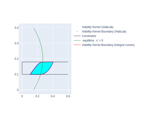
For the parameter values ​​from the article cited above ($r_c=1$, $\delta_c=1$, $a_c=0.3$, $r_s=3$, $s^*=1$, $\alpha_{ws}=0.5$, $u_{min} = -0.02$, $u_{max} = 0.02$, $\underline{g}=0$, $s_{min} = 0.1$, $s_{max} = 0.18$), the viability kernel can be obtained by calculating two integral curves (the authors of the article did not elaborate on this point).

Indeed, its boundary is defined by a closed curve formed by subsets of the boundary of the constraint set $K$ and two integral curves:

• the one originating from the point $(\gamma_g^1,s_{min}) $ with $s'(\gamma_g^1,s_{min})) = 0$ that follows the backward dynamics: 
  \begin{equation}
  \left\{\begin{array}{ll}
  \gamma_g'&= -u_{min}\\
  s'&= -(\frac{r_c}{\delta_c}s(a_c+r_ss)(1-\frac{s}{s^*}-\alpha_{ws})-\gamma_gs)\\ 
  \end{array}\right.
  \end{equation}
• the other originating from the point $(\gamma_g^2,s_{max}) $ with $s'(\gamma_g^2,s_{max})) = 0$ that follows that follows the backward dynamics: 
  \begin{equation}
  \left\{\begin{array}{ll}
  \gamma_g'&= -u_{max}\\
  s'&= -(\frac{r_c}{\delta_c}s(a_c+r_ss)(1-\frac{s}{s^*}-\alpha_{ws})-\gamma_gs)\\ 
  \end{array}\right.
  \end{equation}

The following figure shows the boundary of the viability kernel as a closed curve, along with the approximation obtained using the ViabLab software on a 2001 × 2001 grid of points. The result is consistent with the graph in the original article and is far more precise in the section of the kernel boundary that coincides with the boundary of the constraint set, as well as in the section defined by the integral curves.

This system describes a farm and a restaurant belonging to a same project. Farm production is designed to supply the restaurant, thus minimizing the need of food purchases from external suppliers. Consequently, both activities work in close cooperation, and their respective management must be carefully calibrated in order to maintain the viability of the whole project. More specifically, in the absence of other outlets, any vegetable overproduction would go unused, resulting in the loss of all corresponding production costs. An over-intensive use of the farm plots can also lead to soil depletion, thereby reducing future yields. Conversely, introducing fallow plots helps to maintain soil quality, but an underproduction of vegetables would require a purchase of additional food supply at a high price in order to meet the restaurant's needs. 

This system, and the associated model, are described in the following article : 

de Lapparent, A., Martin, S. & Sabatier, R. Using System Modularity to Simplify Viability Studies: An Application to a Farm-Restaurant Interaction. Environ Model Assess (2024). https://doi.org/10.1007/s10666-024-10014-w

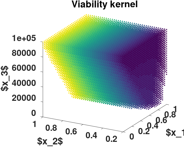
The object computed is a viability kernel. The model is discrete in states, controls and time.

The computation takes a moment (4088s on my computer), be patient...

Model

States and controls

State variables

upper limit of $x_1$ can be relaxed.

Control variables

Dynamics

Overall dynamics are:

\begin{equation}
   \mathcal{S}_U
   \begin{cases}
   x_{1}^{t+1} = x_{1}^t + G(x_{2}^t,u_{3}^t,R(x_3^t,u_1^t,u_2^t)) - E(u_{1}^t,u_{2}^t)\\
   x_{2}^{t+1} = \alpha(x_{2}^t,u_{3}^t,R(x_3^t,u_1^t,u_2^t))\\
   x_{3}^{t+1} = \Phi (x_{3}^t ,u_{1}^t,u_{2}^t) \\
   \end{cases}
\end{equation}

with the following functions:

Some dynamics require to use grid parameters. Consequently, a function has been implemented into the source file to get these values.

Constraints

There are two cconstraints in this system: the global system has to be profitable and a minimal soil quality has to be preserved in order to address sustainability concerns. These constraints take the form of thresholds on the cumulative cash flow ($x_{1} \geq x_{1min}$) and on soil quality ($x_3 \geq x_{3min}$), respectively. In other words, $(x_1^t,x_2^t,x_3^t)$ must remain in $K$ for all $t\in \mathbb{N}$ with : 
\begin{equation}
K:=\{(x_1,x_2,x_3)\in \mathbb{R}^+\times [0;1]^2 \; |\; x_1\geq x_{1min} \text{ and }x_3\geq x_{3min}\}.
\end{equation}

Implementation parameters

Time horizon

The time horizon (for trajectory computations) is 20 years.

Algorithm parameters

Default parameters are used.

System parameters

We used the parameters for a low-hypotheses computation.

   "SYSTEM_PARAMETERS": {
       "DYNAMICS_TYPE": 2,
       "DYN_BOUND": 1,
       "DYN_BOUND_COMPUTE_METHOD": 2,
       "IS_TIMESTEP_GLOBAL": 0,
       "LIPSCHITZ_CONSTANT": 1,
       "LIPSCHITZ_CONSTANT_COMPUTE_METHOD": 2,
       "TIME_DISCRETIZATION_SCHEME": 4
   }

Viability kernel computed using ViabLab