Introduction
The accumulation of nutrients (such as phosphorus or nitrogen) in the water of a lake can lead to a change of state that results in the proliferation of algae, the degradation of water quality and biodiversity, and possibly bacterial blooms: this is eutrophication. The problem of the lake and its riparian holdings is to determine whether it is possible to reconcile the practice of an activity which provides nutrients and the conservation of the lake in a desirable state (oligotrophic, as opposed to eutrophic).
This problem is described in detail in:
S. Martin. The cost of restoration as a way of defining resilience: a viability approach applied to a model of lake eutrophication. Ecol. Soc. http://www.ecologyandsociety.org/vol9/iss2/art8
Nutrients inputs $L$ must be above a minimal threshold $L_{min}$, to take into account the needs of the holdings' activities; And the concentration of total Phosphorus $P$ must remain below a threshold $P_{max}$, to keep the lake in an oligotrophic state. These desirable states form the constraints set $K=[L_{min}, +\infty[ \times [0,P_{max}]$.
The evolution of the concentration of total phosphorus in the lake is modeled by a pseudo-sygmoid:
$$\frac {dP} {dt}=-bP(t)+L(t)+r\frac {P(t)^{q}} {m^{q} + P(t)^{q}} \qquad$$
It is assumed that the evolution of phosphorus inputs can be controlled (by decontamination units, the establishment of wetlands, changes in agricultural or industrial practices, etc.), and we model these controls by a single quantity $u\in U=[u_min,u_max]$. The dynamics of the inputs are modeled by:
$$\frac {dL} {dt}=u \in [- u_{min}, u_{max}] \qquad$$
The viabillity problem is then defined by:
\begin{equation}
(P)\left\{
\begin{array}{l}
\frac{dL}{dt}=u\in U=\left[ u_{min},u_{max}\right] \\
\frac{dP}{dt}=-b P(t) + L(t) +r\frac{P(t)^{q}}{m^{q} + P(t)^{q}} \\
\left(L(t),P(t)\right) \in K=[L_{min}, +\infty[ \times [0,P_{max}]
\end{array}
\right.
\end{equation}
Exemple
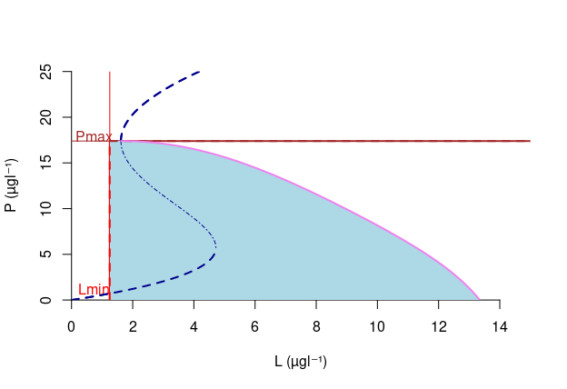
The viabillity kernel can be obtained by calculating an integral curve, starting from the intersection between the boundary of the constraint set and the upper stable curve of equilibrium (see page 7 in https://arxiv.org/pdf/2107.02684 ) and following the backward dynamics. Next figure shows the result for the following parameters: $b=1.95$ an$^{-1}$ ; $q=1.9$ ; $m=19.44\ \mu gl^{-1}$; $r=72.22\ \mu gl^{-1}$ an$^{-1}$; $L_{min}=1.25\ \mu gl^{-1}$ ; $P_{max}=17.39\ \mu gl^{-1}$ ; $|u_{min}|=u_{max}=3.15$.
An approximation can be calculated directly with viability kernel calculation software such as ViabLab.
File .json (to be placed in the following repertory: VIABLAB/INPUT): Lac_params.json
File .h (to be placed in the following repertory: VIABLAB/source/data : data_Lac.h
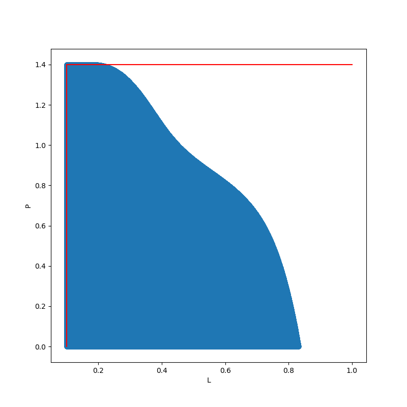
These files correspond to the parameters: $b=0.8$ year$^{-1}$ ; $q=8$ ; $m=1\ \mu gl^{-1}$; $r=1\ \mu gl^{-1}$ year$^{-1}$; $L_{min}=0.1\ \mu gl^{-1}$ ; $P_{max}=1.4\ \mu gl^{-1}$ ; $|u_{min}|=u_{max}=0.09$.
The control is discretized onto 3 values due to the specific characteristics of the problem.
The discretization is performed on 5000 points per axis. The approximation calculated by ViabLab is shown in the following figure. The constraint thresholds are shown in red. It can be seen that the kernel approximation is well performed from the outside.