Social sciences

Language diversity

Niveau de difficulté
Mathematical framework
Continuous time
Continuous space
Viability kernel
Contenu

Introduction

Many languages ​​are at risk of disappearing. It is therefore crucial to understand the mechanisms underlying changes in the number of speakers and to determine if there are measures that could help preserve some of them.

In their article,

Abrams, S. Strogatz, Modelling the dynamics of language death, Nature 424 (6951) (2003) 900

Abrams and Strogatz proposed a mathematical model for studying language competition.

This model fits well with several sets of empirical data: it satisfactorily accounts for historical data concerning the decline of Welsh, Scottish Gaelic, Quechua, and other endangered languages.

In the Abrams and Strogatz model, as well as in those derived from it, the population size is assumed to remain constant. Therefore, the variables are the proportions of the different speaker groups. In models that include bilingualism, the population consists of three groups: monolingual speakers of language A, monolingual speakers of language B, and bilingual speakers AB. The model is two-dimensional, with $\sigma_A$ representing the proportion of speakers of language A and $\sigma_B$ the proportion of speakers of language B ($\sigma_{AB} = 1 - \sigma_A - \sigma_B$).

Within any linguistic subpopulation, forces and influences lead members of one group to switch languages ​​in favor of another. In the Abrams and Strogatz model, the rate at which speakers of one language learn the second language depends on the attractiveness of the latter. In their most general definition of attractiveness, Abrams and Strogatz postulate that a language is more attractive the more speakers it has and the higher its prestige.

In their article,

C. Bernard, S. Martin, Building strategies to ensure language coexistence in presence of bilingualism, Appl. Math. Comput. (2012), doi:10.1016/j.amc.2012.02.041

The authors model only the transitions of the following four types: A → AB, AB → A, A → AB, and AB → B (with the transitions A → B and B → A being extremely rare in practice). They also assume an asymmetry between monolinguals and bilinguals: A → AB (or B → AB) occurs at a rate proportional to the attractiveness of monolingual speakers of A (or B); AB → A (or AB → B) occurs at a rate proportional to the attractiveness of the entire pool of speakers of A, including bilinguals (thus, some bilinguals can become monolingual speakers of A even if A has no monolingual speakers).
Consequently, the two-dimensional model is defined by:

$$
\left\{\begin{array}{ll}
\sigma_A' &= (1-\sigma_A-\sigma_B)(1-\sigma_B)^as_A-\sigma_A\sigma_B^as_B\\
\sigma_B' &= (1-\sigma_A-\sigma_B)(1-\sigma_A)^as_B-\sigma_B\sigma_A^as_A
\end{array}\right.
$$

where $s_A$ (resp. $s_B$) denotes the prestige of language A (resp. B), and $a$ is a parameter modeling how the attractiveness of a language varies with the proportion of its speakers.
For convenience, the authors assume that $s_A+s_B=1$, allowing the substitutions $s_A=s$ and $s_B=1-s$.

The problem of the coexistence of two languages

Bernard and Martin consider that prestige, $s$, can evolve (under the influence of public action, for example), but that its variation at each time step is limited. Thus,

$$
s' = u\in U=[\underline{u};\bar{u}]
$$

When $u>0$, the prestige of language A increases and that of B decreases; the reverse occurs when $u<0$.

The dynamics of the system are thus described by:

$$
\left\{\begin{array}{ll}
\sigma_A' &= (1-\sigma_A-\sigma_B)(1-\sigma_B)^as-\sigma_A\sigma_B^a(1-s)\\
\sigma_B' &= (1-\sigma_A-\sigma_B)(1-\sigma_A)^a(1-s)-\sigma_B\sigma_A^as\\
s' &= u\in U=[\underline{u};\bar{u}]
\end{array}\right.
$$

The authors propose seeking strategies based on prestige variations that ensure the coexistence of the two languages—that is, strategies that maintain a certain level of monolingual speakers for each language. The set of constraints can thus be written as follows:

$$
K:= [\underline{\sigma};1]\times[\underline{\sigma};1]\times [0;1]
$$

Solving this problem means finding the set of states $(\sigma_A, \sigma_B, s)$ from which it is possible to maintain a certain proportion of monolingual groups by manipulating the relative prestige of the two languages—that is, the viability kernel in the terminology of viability theory.


Dynamics Controls Uncertainties Constraints Target Viability Concept

Continuous time

Continuous 3-dimensional space

$
\left\{\begin{array}{ll}
\sigma_A' &= (1-\sigma_A-\sigma_B)(1-\sigma_B)^as-\sigma_A\sigma_B^a(1-s)\\
\sigma_B' &= (1-\sigma_A-\sigma_B)(1-\sigma_A)^a(1-s)-\sigma_B\sigma_A^as\\
s' &= u
\end{array}\right.
$

$(\sigma_A,\sigma_B,s)\in [0;1]\times[0;1]\times [0;1]\cap \{\sigma_A+\sigma_B\leq 1\}
$

Parameter : $a$

$u\in U=[\underline{u};\bar{u}]$

Parameters : $\underline{u},\bar{u}$

None

$
K:= [\underline{\sigma};1]\times[\underline{\sigma};1]\times [0;1]
$


Parameters : $\underline{\sigma}$

None Viability kernel

Results

In the article cited above, the authors provided an analytical description of the viability kernel boundary, composed of integral curves originating from specific points on the boundary of the constraint set.
To illustrate their result, they reproduced the viability kernel for the parameter values ​​$a=1.41$, $\underline{u}=-0.06$, $\bar{u}=0.06$, and $\underline{\sigma}=0.1$.

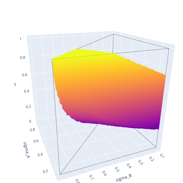
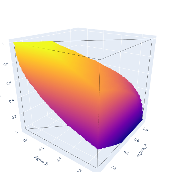
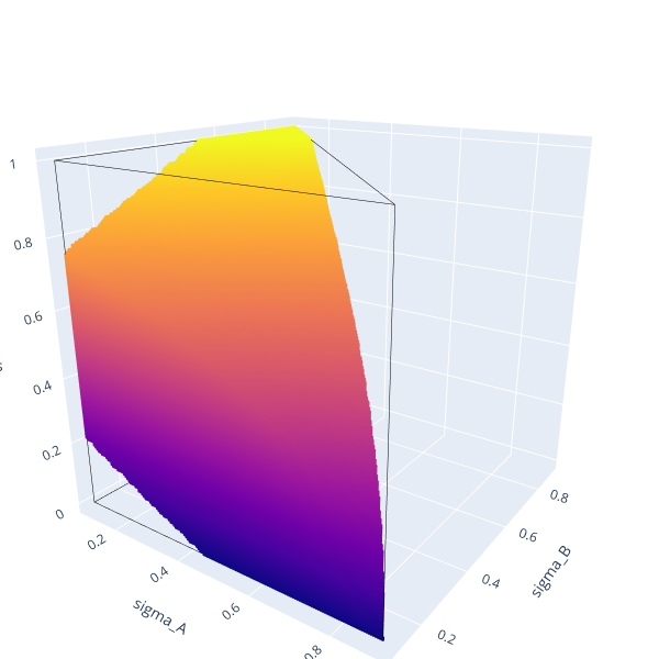
Below, we present four 3D views of the viability kernel approximation corresponding to these parameter values, generated using the ViabLab software based on a $201 \times 201 \times 201$ grid of points (the black lines represent the edges of the constraint set):
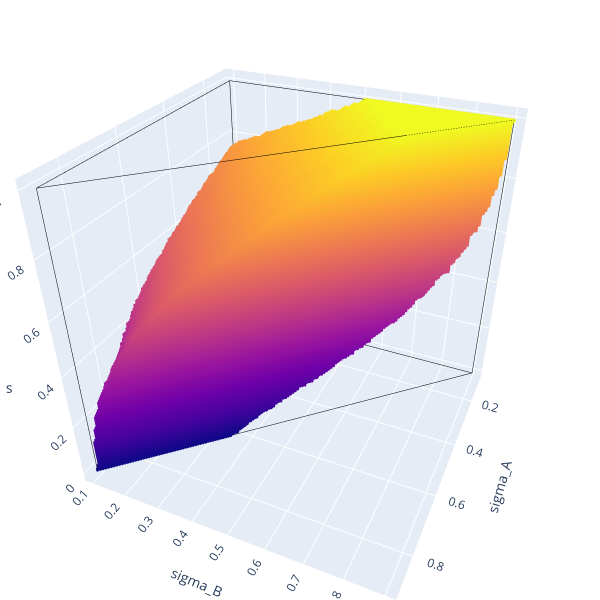
As expected, the kernel is invariant under the transformation $\sigma_A\rightarrow \sigma_B$, $\sigma_B\rightarrow \sigma_A$, and $s\rightarrow 1-s$.

Non-viable situations correspond to states from which:

  • even a continuous increase in the prestige of language A—at maximum intensity—up to its maximum value of 1 would not prevent the proportion of its speakers from crossing the threshold $\underline{\sigma}$,
  • or even a continuous increase in the prestige of language B—at maximum intensity—up to its maximum value of 1 would not prevent the proportion of its speakers from crossing the threshold $\underline{\sigma}$.
Commentaires

We provide the files needed to calculate the aforementioned approximations using the ViabLab software below.

Please consult the training materials:

  • to perform the calculation
  • to understand and visualize the results.

Résilience et changements de régime dans les pêcheries continentales au Sénégal

Niveau de difficulté
Mathematical framework
Discrete space
Discrete time
Contenu

Résumé

Ce travail propose d’explorer comment les concepts de durabilité, de résilience et de changement de régime peuvent être mobilisés dans le cadre de la modélisation et simulation participative (approche ComMod). 

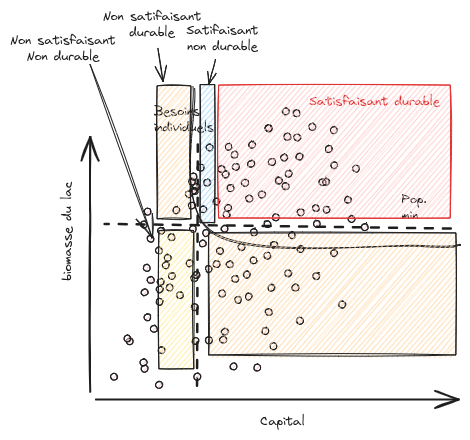
En s’appuyant sur la méthode développée par Mathias et al. (2024) pour identifier les différents régimes d’un modèle stochastique, nous avon adapté ces outils à un modèle multi-agents représentant la pêcherie du lac de Guiers au Sénégal. L’objectif est d’évaluer, comment un système socio-écologique soumis à des incertitudes peut passer d’un état « satisfaisant et durable » à un état « satisfaisant et non-durable » ou « non satisfaisant durable », ou inversement (c.f. fig. 1), selon les conditions définies collectivement avec les parties prenantes.

Au-delà de la mise en œuvre technique, cette étude initie une réflexion sur les enjeux de l'exploration des régimes dans un cadre participatif, où les résultats de la modélisation peuvent déboucher sur des recommandations difficiles — comme une suspension temporaire de la pêche pour préserver la ressource. Elle souligne à la fois le potentiel de ces approches pour structurer le dialogue entre chercheurs et acteurs de terrain, et leurs limites pratiques liées à la complexité des modèles et à la nature stochastique des systèmes étudiés. Ce travail constitue ainsi une première étape vers une intégration concrète des notions de durabilité et de résilience dans les processus de décision collective autour de la gestion durable des pêcheries continentales


Les idées originelles

L’article « From tipping point to tipping set: Extending the concept of regime shift to uncertain dynamics for real-world applications » (Mathias, Deffuant & Brias, Ecological Modelling, 2024) propose une refondation du concept de changement de régime dans les systèmes socio-écologiques. Les auteurs soulignent que la définition classique, basée sur des transitions entre bassins d’attraction dans des systèmes déterministes, devient inadaptée lorsque les dynamiques sont soumises à des perturbations aléatoires. Pour pallier cela, ils introduisent la notion d’ensemble de bascule (tipping set), qui remplace le point de bascule unique. Leur approche s’appuie sur la définition d’un ensemble de satisfaction, correspondant aux états jugés « souhaitables » selon des critères écologiques, économiques ou sociaux, et sur deux indicateurs statistiques : le temps moyen de séjour dans cet ensemble et le temps médian de sortie. Ces mesures permettent de distinguer différents régimes — satisfaction durable, satisfaisant non durable, insatisfaisant durable, insatisfaisant non durable, et résiliente — et de caractériser la stabilité du système en prenant en compte les incertitudes.

Le contexte de l'intervention

Le travail s’inscrit dans le cadre du Living Lab de Mbane initier dans le cadre du projet Santés & Territoires, autour du lac de Guiers au Sénégal, où la pêche constitue à la fois une ressource alimentaire essentielle et un pilier économique pour les communautés locales. Face à la surexploitation des ressources halieutiques et aux pressions environnementales, Nous avons mis en place une démarche de modélisation d’accompagnement (ComMod) visant à co-construire avec les pêcheurs une compréhension partagée du système de pêche pour identifier les marges de manoeuvre d'addapations. Cette approche participative, a permis de co-construire un modèles a base d'agent (avec NetLogo) avec les pêcheurs du lac, qui permet de relier les savoirs locaux aux outils scientifiques. L’objectif est d’aider les acteurs locaux à anticiper les impacts de leurs pratiques et à formuler collectivement des règles de gestion plus robustes et adaptées à leur contexte socio-écologique.

Les résultats

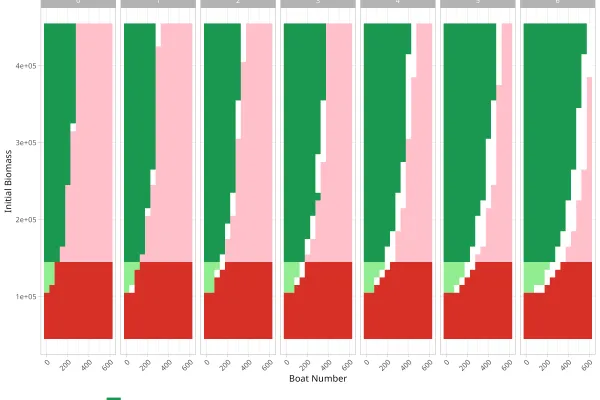
Les résultats de ce travail montrent d’abord la faisabilité technique de l’implémentation des calculs de régimes dans des modèles stochastiques, en s’appuyant sur les travaux de Mathias et al. (2024). Après avoir vérifié la validité de leur approche sur un modèle théorique d’exploitation de ressources naturelles, les auteurs l’appliquent à un modèle multi-agents représentant la pêcherie du lac de Guiers au Sénégal. Les simulations permettent d’identifier différents types de régimes selon des critères de satisfaction définis collectivement : la durabilité économique des pêcheurs (mesurée par leur capital) et la durabilité écologique (liée à la biomasse du lac). Ces exploration révèlent que, dans les conditions simulées, les situations véritablement « satisfaisantes et durables » sont rares : le système tend globalement vers des états non durables, suggérant une vulnérabilité structurelle de la pêcherie face à la pression d’exploitation.

Figure 2 : 

Malgré la portée largement qualitative et exploratoire de ces résultats, le modèle n’étant pas encore calibré sur des données réelles. l'intérêt réside surtout dans la démonstration du potentiel de ces outils pour accompagner les acteurs dans la compréhension des dynamiques complexes de la pêche et dans la formulation de décisions collectives. En particulier, l’identification d’ensembles de bascule — zones d’incertitude entre régimes durables et non durables — offre un support de discussion sur les limites et les risques liés à certaines pratiques. Nous soulignons enfin que ces approches nécessitent un dialogue étroit avec les parties prenantes, car elles peuvent aboutir à des recommandations difficiles, comme la fermeture temporaire de la pêche, tout en constituant une base solide pour articuler modélisation scientifique, participation locale et gestion durable des ressources.


Lake eutrophication and riparian holdings

Niveau de difficulté
Mathematical framework
Continuous time
Continuous space
Viability kernel
Contenu

Introduction

The accumulation of nutrients (such as phosphorus or nitrogen) in the water of a lake can lead to a change of state that results in the proliferation of algae, the degradation of water quality and biodiversity, and possibly bacterial blooms: this is eutrophication. The problem of the lake and its riparian holdings is to determine whether it is possible to reconcile the practice of an activity which provides nutrients and the conservation of the lake in a desirable state (oligotrophic, as opposed to eutrophic).

This problem is described in detail in:

S. Martin. The cost of restoration as a way of defining resilience: a viability approach applied to a model of lake eutrophication. Ecol. Soc.   http://www.ecologyandsociety.org/vol9/iss2/art8

Modeling

Nutrients inputs $L$ must be above a minimal threshold $L_{min}$, to take into account the needs of the holdings' activities; And the concentration of total Phosphorus $P$ must remain  below a threshold  $P_{max}$, to keep the lake in an oligotrophic state. These desirable states form the constraints set $K=[L_{min}, +\infty[ \times [0,P_{max}]$.

The evolution of the concentration of total phosphorus in the lake is modeled by a pseudo-sygmoid:

$$\frac {dP} {dt}=-bP(t)+L(t)+r\frac {P(t)^{q}} {m^{q} + P(t)^{q}} \qquad$$

It is assumed that the evolution of phosphorus inputs can be controlled (by decontamination units, the establishment of wetlands, changes in agricultural or industrial practices, etc.), and we model these controls by a single quantity $u\in U=[u_min,u_max]$. The dynamics of the inputs are modeled by:

$$\frac {dL} {dt}=u \in [- u_{min}, u_{max}] \qquad$$

The viabillity problem is then defined by:

\begin{equation}
(P)\left\{
\begin{array}{l}
\frac{dL}{dt}=u\in U=\left[ u_{min},u_{max}\right] \\
\frac{dP}{dt}=-b P(t) + L(t) +r\frac{P(t)^{q}}{m^{q} + P(t)^{q}} \\
\left(L(t),P(t)\right) \in K=[L_{min}, +\infty[ \times [0,P_{max}]
\end{array}
\right.
\end{equation}
 

Solving this problem means finding the set of states $(L, P)$ from which it is possible to preserve an oligotrophic lake over time while maintaining agricultural activities—that is, the viability kernel in the terminology of viability theory.

Dynamics Controls Uncertainties Constraints Target Viability concept

Continuous time

Continuous 2-dimensional space

\begin{equation}
\left\{
\begin{array}{l}
\frac{dL}{dt}=u\\
\frac{dP}{dt}=-b P(t) + L(t) +r\frac{P(t)^{q}}{m^{q} + P(t)^{q}} 
\end{array}
\right.
\end{equation}

Parameters : $b, r, m, q$

$u\in U=\left[ u_{min},u_{max}\right]$

Parameters : $b, r, m, q$

None

$\left(L(t),P(t)\right) \in K=[L_{min}, +\infty[ \times [0,P_{max}]$


Parameters : $L_{min}, P_{max}$

None Viability kernel

Results

The viability kernel can be obtained by calculating an integral curve (see page 7 of https://arxiv.org/pdf/2107.02684).

Indeed, its boundary is defined by a closed curve formed by subsets of the boundary of the constraint set $K$ and an integral curve originating from the point $(L_e, P_{max})$, where $\frac{dP}{dt}(L_e, P_{max}) = 0$, that follows the backward dynamics:
\begin{equation}
\left\{
\begin{array}{l}
\frac{dL}{dt}=-u_{min}\\
\frac{dP}{dt}=-(-b P(t) + L(t) +r\frac{P(t)^{q}}{m^{q} + P(t)^{q}}) 
\end{array}
\right.
\end{equation}


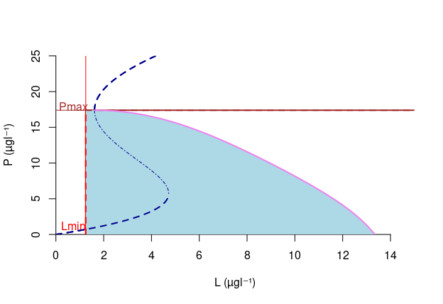
Next figure shows the result for the following parameters:  $b=1.95$ an$^{-1}$ ; $q=1.9$ ; $m=19.44\  \mu gl^{-1}$; $r=72.22\  \mu gl^{-1}$ an$^{-1}$; $L_{min}=1.25\  \mu gl^{-1}$ ; $P_{max}=17.39\  \mu gl^{-1}$ ;   $|u_{min}|=u_{max}=3.15$.

Viability kernel for lake eutrophication problem with integral curve
Viability kernel of the eutrophication lake problem. In light blue the viabillity kernel. The dotted marine line shows the equilibrium curve of the system. In violet the integral curve with $u=u_{min}$.


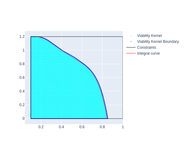
Because the boundary of this viability problem can be described using an integral curve, it is possible to assess the accuracy of approximations generated by generic software.

Shown below the comparison for $b=0.8$ year$^{-1}$ ; $q=8$ ; $m=1\  \mu gl^{-1}$; $r=1\  \mu gl^{-1}$ year$^{-1}$; $L_{min}=0.1\  \mu gl^{-1}$ ; $P_{max}=1.2\  \mu gl^{-1}$ ;   $-u_{min}=u_{max}=0.09$ between the viability kernel defined by the integral curve (in red) and the approximate result obtained using the ViabLab software on a regular 3001×3001 grid (light blue set with a dark blue boundary):

 It can be seen that the kernel approximation is well performed from the outside.


Commentaires

We provide the files needed to calculate the aforementioned approximations using the ViabLab software below.

Please consult the training materials:

  • to perform the calculation
  • to understand and visualize the results.
Fichier(s) de code