Résilience et changements de régime dans les pêcheries continentales au Sénégal
Résumé
Ce travail propose d’explorer comment les concepts de durabilité, de résilience et de changement de régime peuvent être mobilisés dans le cadre de la modélisation et simulation participative (approche ComMod).
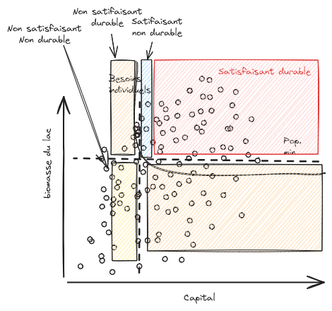
En s’appuyant sur la méthode développée par Mathias et al. (2024) pour identifier les différents régimes d’un modèle stochastique, nous avon adapté ces outils à un modèle multi-agents représentant la pêcherie du lac de Guiers au Sénégal. L’objectif est d’évaluer, comment un système socio-écologique soumis à des incertitudes peut passer d’un état « satisfaisant et durable » à un état « satisfaisant et non-durable » ou « non satisfaisant durable », ou inversement (c.f. fig. 1), selon les conditions définies collectivement avec les parties prenantes.
Au-delà de la mise en œuvre technique, cette étude initie une réflexion sur les enjeux de l'exploration des régimes dans un cadre participatif, où les résultats de la modélisation peuvent déboucher sur des recommandations difficiles — comme une suspension temporaire de la pêche pour préserver la ressource. Elle souligne à la fois le potentiel de ces approches pour structurer le dialogue entre chercheurs et acteurs de terrain, et leurs limites pratiques liées à la complexité des modèles et à la nature stochastique des systèmes étudiés. Ce travail constitue ainsi une première étape vers une intégration concrète des notions de durabilité et de résilience dans les processus de décision collective autour de la gestion durable des pêcheries continentales
Les idées originelles
L’article « From tipping point to tipping set: Extending the concept of regime shift to uncertain dynamics for real-world applications » (Mathias, Deffuant & Brias, Ecological Modelling, 2024) propose une refondation du concept de changement de régime dans les systèmes socio-écologiques. Les auteurs soulignent que la définition classique, basée sur des transitions entre bassins d’attraction dans des systèmes déterministes, devient inadaptée lorsque les dynamiques sont soumises à des perturbations aléatoires. Pour pallier cela, ils introduisent la notion d’ensemble de bascule (tipping set), qui remplace le point de bascule unique. Leur approche s’appuie sur la définition d’un ensemble de satisfaction, correspondant aux états jugés « souhaitables » selon des critères écologiques, économiques ou sociaux, et sur deux indicateurs statistiques : le temps moyen de séjour dans cet ensemble et le temps médian de sortie. Ces mesures permettent de distinguer différents régimes — satisfaction durable, satisfaisant non durable, insatisfaisant durable, insatisfaisant non durable, et résiliente — et de caractériser la stabilité du système en prenant en compte les incertitudes.
Le contexte de l'intervention
Le travail s’inscrit dans le cadre du Living Lab de Mbane initier dans le cadre du projet Santés & Territoires, autour du lac de Guiers au Sénégal, où la pêche constitue à la fois une ressource alimentaire essentielle et un pilier économique pour les communautés locales. Face à la surexploitation des ressources halieutiques et aux pressions environnementales, Nous avons mis en place une démarche de modélisation d’accompagnement (ComMod) visant à co-construire avec les pêcheurs une compréhension partagée du système de pêche pour identifier les marges de manoeuvre d'addapations. Cette approche participative, a permis de co-construire un modèles a base d'agent (avec NetLogo) avec les pêcheurs du lac, qui permet de relier les savoirs locaux aux outils scientifiques. L’objectif est d’aider les acteurs locaux à anticiper les impacts de leurs pratiques et à formuler collectivement des règles de gestion plus robustes et adaptées à leur contexte socio-écologique.
Les résultats
Les résultats de ce travail montrent d’abord la faisabilité technique de l’implémentation des calculs de régimes dans des modèles stochastiques, en s’appuyant sur les travaux de Mathias et al. (2024). Après avoir vérifié la validité de leur approche sur un modèle théorique d’exploitation de ressources naturelles, les auteurs l’appliquent à un modèle multi-agents représentant la pêcherie du lac de Guiers au Sénégal. Les simulations permettent d’identifier différents types de régimes selon des critères de satisfaction définis collectivement : la durabilité économique des pêcheurs (mesurée par leur capital) et la durabilité écologique (liée à la biomasse du lac). Ces exploration révèlent que, dans les conditions simulées, les situations véritablement « satisfaisantes et durables » sont rares : le système tend globalement vers des états non durables, suggérant une vulnérabilité structurelle de la pêcherie face à la pression d’exploitation.
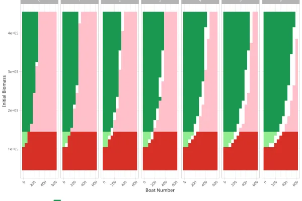
Malgré la portée largement qualitative et exploratoire de ces résultats, le modèle n’étant pas encore calibré sur des données réelles. l'intérêt réside surtout dans la démonstration du potentiel de ces outils pour accompagner les acteurs dans la compréhension des dynamiques complexes de la pêche et dans la formulation de décisions collectives. En particulier, l’identification d’ensembles de bascule — zones d’incertitude entre régimes durables et non durables — offre un support de discussion sur les limites et les risques liés à certaines pratiques. Nous soulignons enfin que ces approches nécessitent un dialogue étroit avec les parties prenantes, car elles peuvent aboutir à des recommandations difficiles, comme la fermeture temporaire de la pêche, tout en constituant une base solide pour articuler modélisation scientifique, participation locale et gestion durable des ressources.
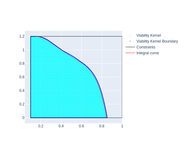
We provide the files needed to calculate the aforementioned approximations using the ViabLab software below.
Please consult the training materials: