Beginner

Viability Theory

Type de document
Editeur
Birkhäuser
Lieu
Boston
Année de publication
1991
Sous titre
Systems & Control: Formations & Applications
Auteur(s)
Jean-Pierre Aubin
Niveau de difficulté
Identifiant
ISBN : 978-1-4612-0451-8
photo

This work examines viability theory and its applications to control theory and differential games. The emphasis is on the construction of feedbacks and dynamical systems by myopic optimization methods. Systems of first-order partial differential inclusions, whose solutions are feedbacks, are constructed and investigated. Basic results are then extended to the case of fuzzy control problems, distributed control problems, and control systems with delays and memory. Aimed at graduate students and research mathematicians, both pure and applied, this book offers specialists in control and nonlinear systems tools to take into account general state constraints. Viability theory also allows researchers in other disciplines—artificial intelligence, economics, game theory, theoretical biology, population genetics, cognitive sciences—to go beyond deterministic models by studying them in a dynamical or evolutionary perspective in an uncertain environment. The book is a compendium of the state of knowledge about viability...Mathematically, the book should be accessible to anyone who has had basic graduate courses in modern analysis and functional analysis…The concepts are defined and many proofs of the requisite results are reproduced here, making the present book essentially self-contained. —Bulletin of the AMS Because of the wide scope, the book is an ideal reference for people encountering problems related to viability theory in their research…It gives a very thorough mathematical presentation. Very useful for anybody confronted with viability constraints. —Mededelingen van het Wiskundig

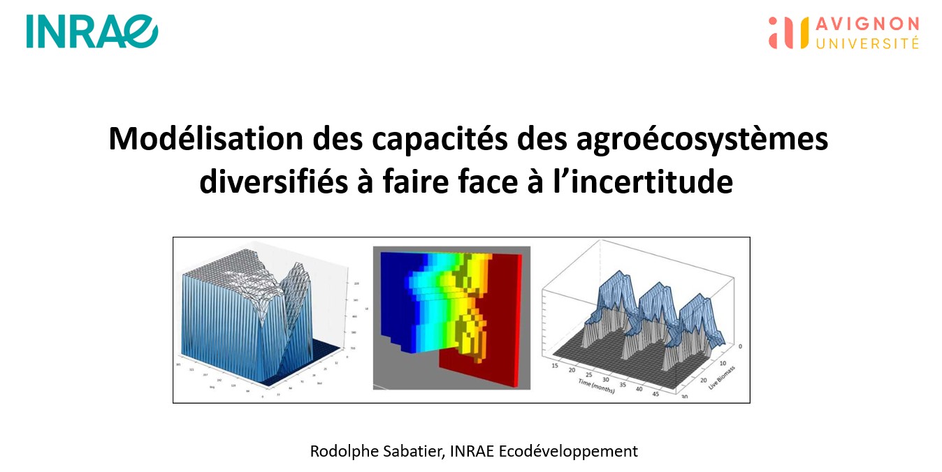
Modélisation des capacités des agrosystèmes diversifiés à faire face à l’incertitude

Type de document
Lieu
Avignon
Année de publication
2025
Sous titre
HDR
Auteur(s)
Rodolphe Sabatier
Niveau de difficulté
schéma

En remettant les processus écologiques au cœur des dynamiques de production, les systèmes agricoles écologisés doivent composer avec de nombreuses incertitudes. La résilience, l’adaptabilité et la flexibilité deviennent alors des propriétés clefs de ces systèmes. En m’appuyant sur les développements récents du cadre mathématique de la Théorie de la viabilité que j’applique à neuf cas d’étude en productions végétales et animales, je propose ici un cadre formel pour l’évaluation de ces propriétés via des méthodes numériques. Ces travaux montrent en quoi se détacher d’une logique d’optimisation monocritère est d’autant plus pertinent que l’on s’intéresse à des systèmes écologisés, c’est-à-dire complexes, évolutifs et aux dynamiques incertaines par nature. Appréhender la viabilité de ces systèmes, demande alors non seulement de considérer leur structure (les états) mais aussi la gamme d’options de pilotage disponibles (les contrôles) permettant de se maintenir dans une gamme de situations jugées acceptables (viables) par l’agriculteur. 

Cela peut impliquer d’élargir le regard porté sur le système étudié en prenant en compte l’ensemble des composantes embarquées par les objectifs de l’agriculteur, quitte à dépasser le cadre agricole strict. De la même manière cet élargissement de point de vue amène à considérer le système agricole dans son environnement en intégrant les interactions avec les autres acteurs du territoire. Ces changements d’échelle que j’envisagerai dans la suite de mes recherches engagent des questions méthodologiques pour continuer à appliquer le cadre de la viabilité à des systèmes plus vastes (de plus grandes dimensions), mais aussi pour en transposer les concepts principaux à des approches plus qualitatives. 

Intégrer l’adaptabilité dans l’analyse de la durabilité des exploitations apicoles

Type de document
Revue
Innovations Agronomiques
Année de publication
2019
Auteur(s)
Kouchner, C., Sabatier, R., Basso, B., Decourtye A., Ferrus C., Le Conte Y., Tchamitchian M.
Niveau de difficulté
Identifiant
10.15454/k4kv-k303
shéma

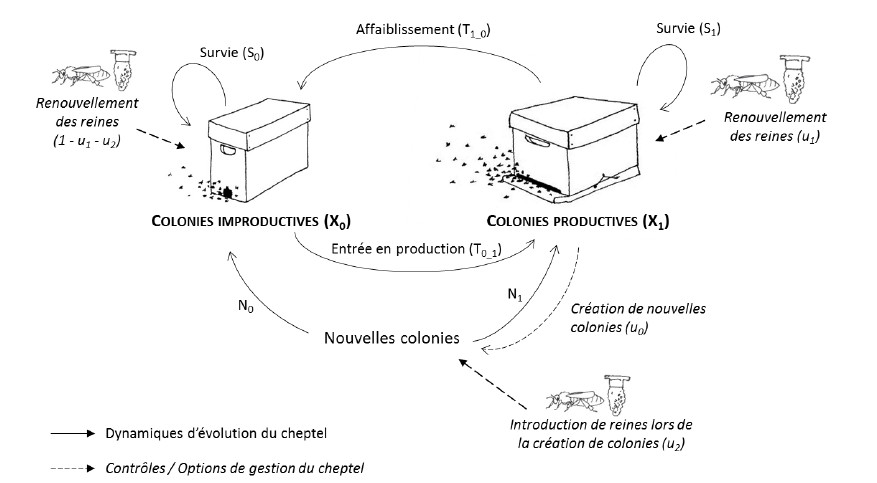
À l’échelle d’une exploitation apicole, la capacité d’adaptation est liée à différents aspects du fonctionnement : aux pratiques de gestion du cheptel, à des choix de commercialisation ou d’organisation. Cette capacité d’adaptation contribue à la durabilité de l’exploitation en lui permettant de composer avec un contexte variable, mais constitue également un élément de plus à considérer dans les compromis à trouver entre plusieurs enjeux de durabilité qui peuvent être antagonistes : viabilité économique, temps de travail… Pour révéler les difficultés possibles à concilier ces différents objectifs avec celui d’adaptabilité dans la gestion du renouvellement du cheptel, nous avons appliqué la théorie de la viabilité à une modélisation des principales options de gestion du renouvellement (gestion des reines, création de nouvelles colonies) et des dynamiques d’évolution du cheptel. Le modèle développé a permis d’étudier les conséquences de différentes pratiques sur la possibilité pour l’exploitation d’atteindre ses objectifs économiques et de temps de travail tout en maintenant un certain niveau d’adaptabilité. Certains choix techniques comme le nombre de reines disponibles (relativement au nombre de colonies de l’exploitation) apparaissent ainsi limiter en amont les options possibles de gestion du cheptel, voire la viabilité de l’exploitation dans certaines situations. L’adaptabilité de la gestion du cheptel apparaît donc comme une contrainte

Julia Sets

Niveau de difficulté
Domain
Mathematical framework
Discrete time
Continuous space
Contenu

Let us consider complex quadratic polynomials that can be expressed as 

$$\phi_c(z)=z^2+c.$$

The filled Julia set gathers $z$ such that the sequence of their iterates by $\phi_c$ is bounded. 

Fix some $R>0$ large enough that $R^2-R\geq |c|$, the filled Julia set for this system is the subset of the complex plane given by

$$K(\phi_c)=\{z\in C\; :\; \forall n \in N, \;|\phi_c^n(z)|\leq R\},$$ 

where $\phi_c^n(z)$ is the nth iterate of $\phi_c(z)$. The Julia set $J(\phi_c)$ of this function is the boundary of $K(\phi_c)$.

In 1982, a deep theorem by Adrien Douady and Hubbard states that Julia sets are path-connected if and only if the sequence of the iterates of $0$ is bounded. 

Moreover, $K(\phi_c)$ and $J(\phi_c)$ are either path-connected (there is a path within the set that connects any two given points in the set) or path-disconnected (for any two given points in the set, it is impossible to find a path within the set that connects the pair). The set of complex numbers $c$ that can form a path-connected Julia set is called the Mandelbrot set. It is defined in the complex plane as the complex numbers $c$ for which the function $\phi_c$ does not diverge to infinity when iterated starting at $z=0$.

The set Mandelbrot set is bounded, included in $B(0,2)$. Different components of the Mandelbrot set correspond to different dynamical behaviors of the corresponding filled Julia sets.


From

Aubin, J.-P., Bayen, A., & Saint-Pierre, P. Viability Theory: New Directions. Springer. 2011.

  • Obviously, the subset $K_c:=Viab_{\phi_c}(B(0,2))$ is the filled Julia set for the function $\phi_c$ whenever $|c|\leq 2$ (which is true when $c$ belongs to the Mandelbrot set) and its boundary $J_u:=\partial K_c$ is the Julia set.

We can approximate these Julia sets thanks to the Viability Algorithm.

Dynamics Controls Uncertainties Constraints Target Viability Concept

Discrete Time

Continous 2-dimensional space

$\phi(x,y):=(x^2-y^2+a,2xy+b)$

Parameters : $a$, $b$ 

None None B(0,2) None Viability Kernel

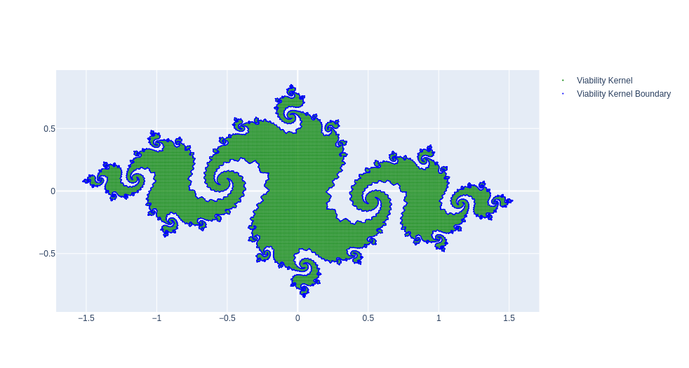
See below approximations of famous Julia sets : 

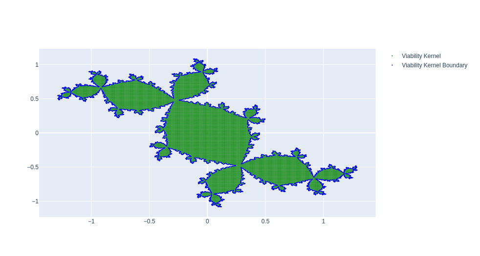
  • Douady Rabbit when $c$ is a complex root of $c^3+2c^2+c+$,  $c\approx -0.123 \pm 0.745i $ which implies that the orbit of 0 is periodic with period 3. Douady Rabbit is then connected. See below an approximation obtained by the ViabLab software with $c=-0.123 + 0.745i$ : 


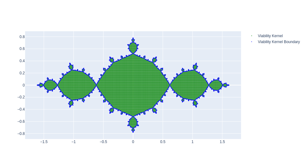
  • An approximation of the famous Basilica when $c=-1$ : 

  • And an approximation of another beautiful Julia set for $c=-0.8+0.156i$ obtained using the VIABLAB software:


Commentaires

We provide below the files necessary to compute the above approximations thans to ViabLab software.

Please refer to training material :

  • to run the computation
  • to understand and visualize the results.


Prey-predator model

Niveau de difficulté
Domain
Mathematical framework
Continuous space
Viability kernel
Continuous time
Contenu

Introduction

Let us consider the classic Lotka-Volterra predator-prey model with two variables: $x(t)$, the prey population size over time, and $y(t)$, the predator population size over time.
Population changes over time depend on:

  • the prey reproduction rate, $\alpha$
  • the prey mortality rate due to predators, $\beta$
  • the predator production rate based on prey consumed, $\delta$
  • the predator mortality rate, $\gamma$.

Lotka and Volterra independently proposed the following equations:

$$\left\{\begin{array}{l}x'=x(\alpha-\beta y)\\ y'=y(\delta x-\gamma)\end{array}\right.$$

Modeling a viability problem for the prey

In their article

Térence Bayen, Alain Rapaport. Minimal time crisis versus minimum time to reach a viability kernel: a case study in the prey-predator model. Optimal Control Applications and Methods, 2019, 40 (2), pp.330-350. ⟨10.1002/oca.2484⟩. ⟨hal-01943636v2⟩

the authors addressed the problem of preserving the prey population in the face of predators by keeping their numbers above a given threshold $\underline{x} > 0$ as much as possible. This amounts to ensuring that the state remains within the set

$$K(\underline{x}):=\{(x,y)\,|\, x>=\underline{x}\},$$

based on the premise that low prey density exposes the population to a risk of extinction that should be avoided as much as possible.

Using the original Lotka-Volterra equations, the authors assume constant values ​​for $\alpha=r$, $\beta=1$, and $\delta=1$. However, a control can influence predator mortality; thus, the authors set $\gamma = m + u$, where $m$ is a constant and $u$ is an excess mortality rate that can vary, with $u(t) \in [0, \bar{u}]$.

The viability problem can be summarized as follows:

\begin{equation}
\left\{
\begin{array}{l}
x'=x(r- y)\\
y'=y( x-m-u)\\
u(t) \in [0;\bar{u}]\\
\left(x(t),y(t)\right) \in K(\underline{x}):=\{(x,y)\,|\, x>=\underline{x}\}
\end{array}
\right.
\end{equation}

Solving this problem means finding the set of states $(x,y)$ from which it is possible to maintain a prey population level above $\underline{x}$ over time by manipulating prey excess mortality—in other words, the viability kernel, using the terminology of viability theory.

Dynamics Controls Uncertainties Constraints Target Viability concept

Continuous time

Continuous in 2D space

\begin{equation}
\left\{
\begin{array}{l}
x'=x(r- y)\\ 
y'=y( x-m-u)\\
\end{array}
\right.
\end{equation}

Parameters : $r, m$

$u\in U=\left[ 0,\bar{u}\right]$

Parameters : $\bar{u}$

None

$\{(x,y)\,|\, x>=\underline{x}\}$


Parameters : $\underline{x}$

None Viability kernel

Results

The authors provide an analytical description of this viability kernel. When $\bar{u}\geq \underline{x}-m$, by considering the invariant of this Lotka-Volterra system (which depends on $u$), $W_u(x,y):=x-(m+u)\ln x+y -r\ln y$, they construct the boundary of the viability kernel using a closed curve composed of three subsets:

  • $\{(x,y) | y\geq r \text{ and }W_{\bar{u}}(x,y)=W_{\bar{u}}(\underline{x}, r) \}$.
  • Let $x^+>\underline{x}$ such that $W_{\bar{u}}(x^+,r)=W_{\bar{u}}(\underline{x}, r)$,
    $\{(x,y) | y\leq r \text{ and }W_{0}(x,y)=W_{0}(x^+, r) \}$
  • Let $r^-$ such that $W_{0}(\underline{x},r^-)=W_{0}(x^+, r)$,
    $\{(x,y) | x=\underline{x} \text{ and } y\in [r^-,r]\}$

The following figure shows the result for the parameters: $r=1$, $m=1$, $\bar{u}=0.5$, $\underline{x}=0.8$.
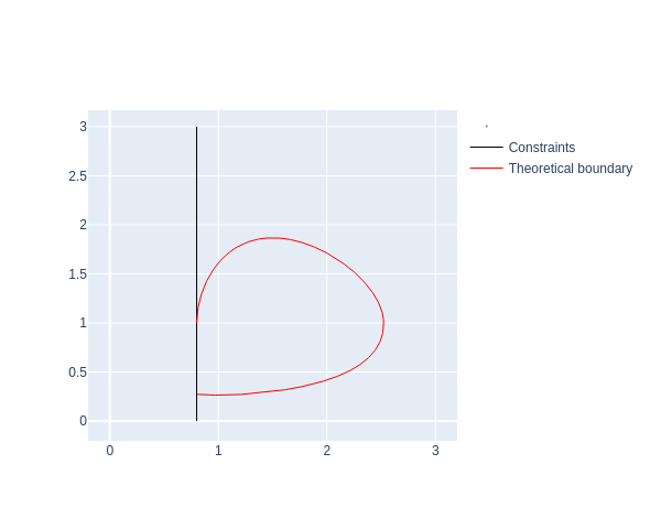
Because an analytical description of its boundary exists, this viability problem allows for testing the precision of approximations generated by generic software.

Shown below is a comparison—for $r=1$, $m=1$, $\bar{u}=0.5$, and $\underline{x}=0.8$—between the viability kernel boundary derived from its analytical description (in red) and the approximate result obtained using the ViabLab software on a regular grid of 4001×4001 points (light blue set with a dark blue boundary):
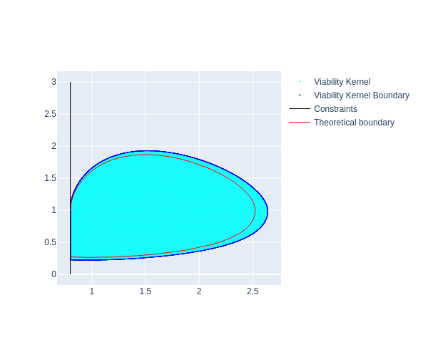
 It can be seen that the kernel approximation is well performed from the outside.

 

Commentaires

We provide the files needed to calculate the aforementioned approximations using the ViabLab software below.

Please consult the training materials:

  • to perform the calculation
  • to understand and visualize the results.
Fichier(s) de code

Rotational grazing of dairy cattle in Wisconsin (USA)

Niveau de difficulté
Domain
Mathematical framework
Discrete space
Discrete time
Contenu

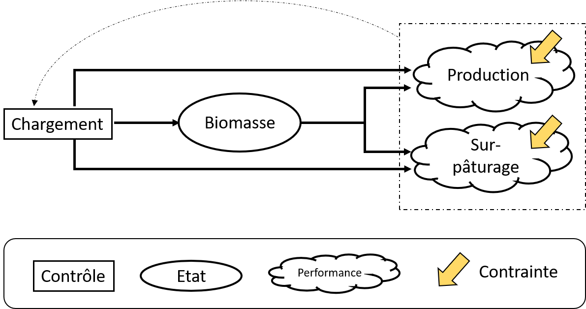
Grass is a renewable resource whose growth rate depends on the time of year, its height, and weather conditions. Effective pasture management therefore requires dynamically setting the stocking rate (number of animals per hectare) to feed the animals while avoiding overgrazing. Due to the uncertainty surrounding grass growth linked to weather conditions, the challenge is to implement grazing schedules that are not only productive but also robust and adaptable.

This problem is described in detail in:

Sabatier R, Oates, LG, Jackson RD, 2015, Management flexibility of a grassland agroecosystem: A modeling approach based on viability theory, Agricultural Systems http://dx.doi.org/10.1016/j.agsy.2015.06.008

The system is characterized by:

  • two states: $X(t)$, the biomass of the grass resource, and $P(t)$, the cumulative production level.
  • a control $U(t)$, the loading rate.
  • an uncertainty ω ∈ Ω on the grass growth rate.


Due to the daily time step of the loading management, the model is discretized in time. Furthermore, since the cows are removed from the paddocks for several consecutive months in winter, the focus is on a single grazing season, which implies a finite time horizon, t ∈ [90, 300].


The dynamics are as follows:


With $r(t, ω)$ the grass growth rate, $K(t)$ a saturation coefficient, $Xmin$ the grass biomass corresponding to the minimum grazing height (cows are unable to graze grass below a certain height), and q the amount of biomass grazed per cow per day.

Two constraints are defined:

  • A constraint aimed at preventing overgrazing: $qU(t) \leq X(t)−Xmin$
  • A constraint aimed at ensuring a minimum level of production over the season P(T) ≥ Pmin

Values of model parameters :

  •  saturation coefficient $K$ and growth coefficient $r$ depend on time and take the successive values of the corresponding vectors at times 90, 105, 140, 200, 251, 280, and 320 ; 


t 90 105 140 200 251 280 320
K 382.14 423.81 894.21 1573.0 750.83 882.0 152.86
r 1.07 1.11 1.07 1.04 1.06 1.05 1.0


  • $q$ is the daily feed intake by cattle, $q = 14.3$;
  • and $w$ is a multiplying coefficient that reflects the daily weather variation, $w \in [0.95; 1.0; 1.05]$.
     

Viabic

Niveau de difficulté
Contenu

But du projet

Trouver pour chaque individu son ensemble d'engagements préservant la viabilité de chacun. Un ensemble d'engagements individuel corresponds à l'ensemble des contrôles (actions min à max, supposées continues) que l'individu peut exercer.

Code

Le code est disponible sur la forge INRAE. Les supports de présentation de viabic sont disponibles sur HAL.

La résolution du problème (ie trouver les bornes des ensembles d'engagements individuels) s'appuie sur une optimisation par essaim particulaire (PSO - Particle Swarm Optimization).