Continuous space

Let us consider complex quadratic polynomials that can be expressed as 

$$\phi_c(z)=z^2+c.$$

The filled Julia set gathers $z$ such that the sequence of their iterates by $\phi_c$ is bounded. 

Fix some $R>0$ large enough that $R^2-R\geq |c|$, the filled Julia set for this system is the subset of the complex plane given by

$$K(\phi_c)=\{z\in C\; :\; \forall n \in N, \;|\phi_c^n(z)|\leq R\},$$ 

where $\phi_c^n(z)$ is the nth iterate of $\phi_c(z)$. The Julia set $J(\phi_c)$ of this function is the boundary of $K(\phi_c)$.

In 1982, a deep theorem by Adrien Douady and Hubbard states that Julia sets are path-connected if and only if the sequence of the iterates of $0$ is bounded. 

Moreover, $K(\phi_c)$ and $J(\phi_c)$ are either path-connected (there is a path within the set that connects any two given points in the set) or path-disconnected (for any two given points in the set, it is impossible to find a path within the set that connects the pair). The set of complex numbers $c$ that can form a path-connected Julia set is called the Mandelbrot set. It is defined in the complex plane as the complex numbers $c$ for which the function $\phi_c$ does not diverge to infinity when iterated starting at $z=0$.

The set Mandelbrot set is bounded, included in $B(0,2)$. Different components of the Mandelbrot set correspond to different dynamical behaviors of the corresponding filled Julia sets.

From

Aubin, J.-P., Bayen, A., & Saint-Pierre, P. Viability Theory: New Directions. Springer. 2011.

• Obviously, the subset $K_c:=Viab_{\phi_c}(B(0,2))$ is the filled Julia set for the function $\phi_c$ whenever $|c|\leq 2$ (which is true when $c$ belongs to the Mandelbrot set) and its boundary $J_u:=\partial K_c$ is the Julia set.

We can approximate these Julia sets thanks to the Viability Algorithm.

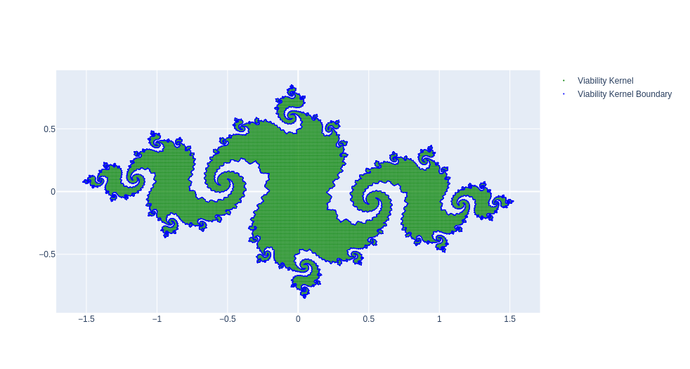
See below approximations of famous Julia sets : 

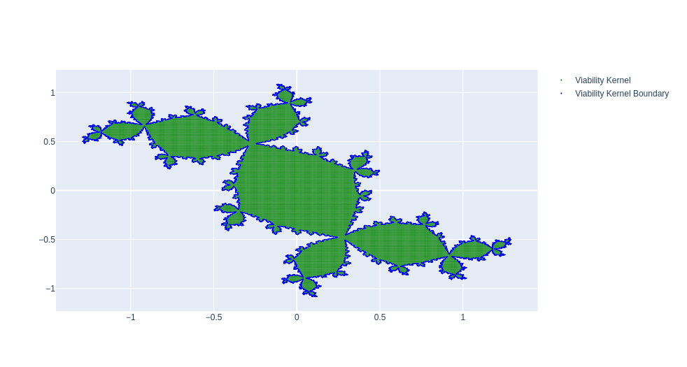
• Douady Rabbit when $c$ is a complex root of $c^3+2c^2+c+$,  $c\approx -0.123 \pm 0.745i $ which implies that the orbit of 0 is periodic with period 3. Douady Rabbit is then connected. See below an approximation obtained by the ViabLab software with $c=-0.123 + 0.745i$ : 

• An approximation of the famous Basilica when $c=-1$ : 

  

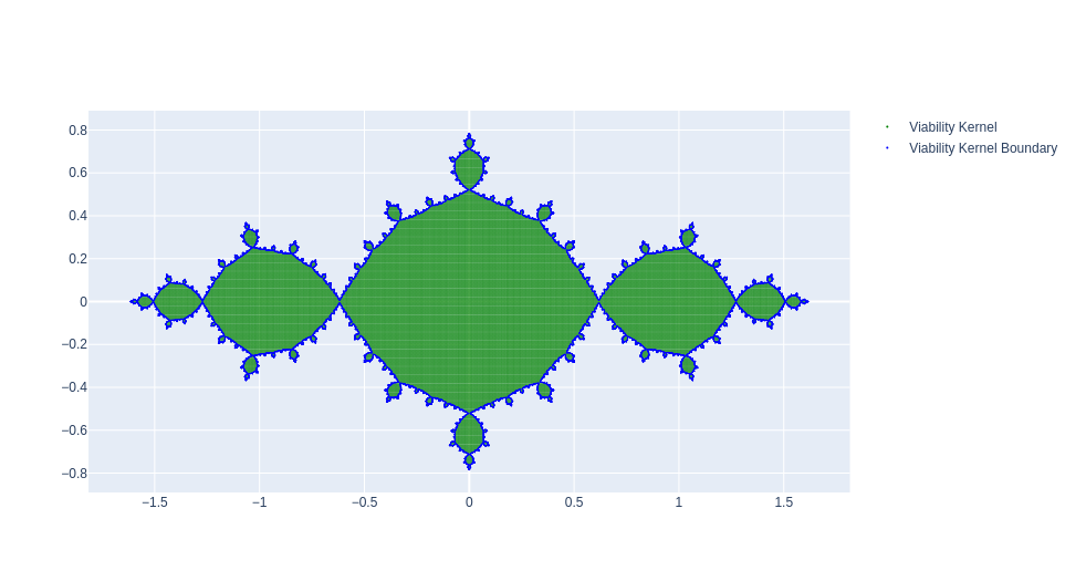
• And an approximation of another beautiful Julia set for $c=-0.8+0.156i$ obtained using the VIABLAB software:

Introduction

Let us consider the classic Lotka-Volterra predator-prey model with two variables: $x(t)$, the prey population size over time, and $y(t)$, the predator population size over time.
Population changes over time depend on:

• the prey reproduction rate, $\alpha$
• the prey mortality rate due to predators, $\beta$
• the predator production rate based on prey consumed, $\delta$
• the predator mortality rate, $\gamma$.

Lotka and Volterra independently proposed the following equations:

$$\left\{\begin{array}{l}x'=x(\alpha-\beta y)\\ y'=y(\delta x-\gamma)\end{array}\right.$$

Modeling a viability problem for the prey

In their article

Térence Bayen, Alain Rapaport. Minimal time crisis versus minimum time to reach a viability kernel: a case study in the prey-predator model. Optimal Control Applications and Methods, 2019, 40 (2), pp.330-350. ⟨10.1002/oca.2484⟩. ⟨hal-01943636v2⟩

the authors addressed the problem of preserving the prey population in the face of predators by keeping their numbers above a given threshold $\underline{x} > 0$ as much as possible. This amounts to ensuring that the state remains within the set

$$K(\underline{x}):=\{(x,y)\,|\, x>=\underline{x}\},$$

based on the premise that low prey density exposes the population to a risk of extinction that should be avoided as much as possible.

Using the original Lotka-Volterra equations, the authors assume constant values ​​for $\alpha=r$, $\beta=1$, and $\delta=1$. However, a control can influence predator mortality; thus, the authors set $\gamma = m + u$, where $m$ is a constant and $u$ is an excess mortality rate that can vary, with $u(t) \in [0, \bar{u}]$.

The viability problem can be summarized as follows:

\begin{equation}
\left\{
\begin{array}{l}
x'=x(r- y)\\
y'=y( x-m-u)\\
u(t) \in [0;\bar{u}]\\
\left(x(t),y(t)\right) \in K(\underline{x}):=\{(x,y)\,|\, x>=\underline{x}\}
\end{array}
\right.
\end{equation}

Solving this problem means finding the set of states $(x,y)$ from which it is possible to maintain a prey population level above $\underline{x}$ over time by manipulating prey excess mortality—in other words, the viability kernel, using the terminology of viability theory.

Results

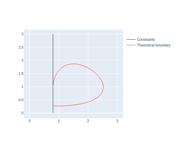
The authors provide an analytical description of this viability kernel. When $\bar{u}\geq \underline{x}-m$, by considering the invariant of this Lotka-Volterra system (which depends on $u$), $W_u(x,y):=x-(m+u)\ln x+y -r\ln y$, they construct the boundary of the viability kernel using a closed curve composed of three subsets:

• $\{(x,y) | y\geq r \text{ and }W_{\bar{u}}(x,y)=W_{\bar{u}}(\underline{x}, r) \}$.
• Let $x^+>\underline{x}$ such that $W_{\bar{u}}(x^+,r)=W_{\bar{u}}(\underline{x}, r)$,
  $\{(x,y) | y\leq r \text{ and }W_{0}(x,y)=W_{0}(x^+, r) \}$
• Let $r^-$ such that $W_{0}(\underline{x},r^-)=W_{0}(x^+, r)$,
  $\{(x,y) | x=\underline{x} \text{ and } y\in [r^-,r]\}$

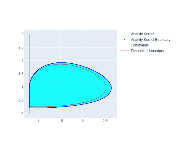
The following figure shows the result for the parameters: $r=1$, $m=1$, $\bar{u}=0.5$, $\underline{x}=0.8$.

Because an analytical description of its boundary exists, this viability problem allows for testing the precision of approximations generated by generic software.

Shown below is a comparison—for $r=1$, $m=1$, $\bar{u}=0.5$, and $\underline{x}=0.8$—between the viability kernel boundary derived from its analytical description (in red) and the approximate result obtained using the ViabLab software on a regular grid of 4001×4001 points (light blue set with a dark blue boundary):

 It can be seen that the kernel approximation is well performed from the outside.

Introduction

The accumulation of nutrients (such as phosphorus or nitrogen) in the water of a lake can lead to a change of state that results in the proliferation of algae, the degradation of water quality and biodiversity, and possibly bacterial blooms: this is eutrophication. The problem of the lake and its riparian holdings is to determine whether it is possible to reconcile the practice of an activity which provides nutrients and the conservation of the lake in a desirable state (oligotrophic, as opposed to eutrophic).

This problem is described in detail in:

S. Martin. The cost of restoration as a way of defining resilience: a viability approach applied to a model of lake eutrophication. Ecol. Soc.   http://www.ecologyandsociety.org/vol9/iss2/art8

Modeling

Nutrients inputs $L$ must be above a minimal threshold $L_{min}$, to take into account the needs of the holdings' activities; And the concentration of total Phosphorus $P$ must remain  below a threshold  $P_{max}$, to keep the lake in an oligotrophic state. These desirable states form the constraints set $K=[L_{min}, +\infty[ \times [0,P_{max}]$.

The evolution of the concentration of total phosphorus in the lake is modeled by a pseudo-sygmoid:

$$\frac {dP} {dt}=-bP(t)+L(t)+r\frac {P(t)^{q}} {m^{q} + P(t)^{q}} \qquad$$

It is assumed that the evolution of phosphorus inputs can be controlled (by decontamination units, the establishment of wetlands, changes in agricultural or industrial practices, etc.), and we model these controls by a single quantity $u\in U=[u_min,u_max]$. The dynamics of the inputs are modeled by:

$$\frac {dL} {dt}=u \in [- u_{min}, u_{max}] \qquad$$

The viabillity problem is then defined by:

\begin{equation}
(P)\left\{
\begin{array}{l}
\frac{dL}{dt}=u\in U=\left[ u_{min},u_{max}\right] \\
\frac{dP}{dt}=-b P(t) + L(t) +r\frac{P(t)^{q}}{m^{q} + P(t)^{q}} \\
\left(L(t),P(t)\right) \in K=[L_{min}, +\infty[ \times [0,P_{max}]
\end{array}
\right.
\end{equation}
 

Solving this problem means finding the set of states $(L, P)$ from which it is possible to preserve an oligotrophic lake over time while maintaining agricultural activities—that is, the viability kernel in the terminology of viability theory.

Results

The viability kernel can be obtained by calculating an integral curve (see page 7 of https://arxiv.org/pdf/2107.02684).

Indeed, its boundary is defined by a closed curve formed by subsets of the boundary of the constraint set $K$ and an integral curve originating from the point $(L_e, P_{max})$, where $\frac{dP}{dt}(L_e, P_{max}) = 0$, that follows the backward dynamics:
\begin{equation}
\left\{
\begin{array}{l}
\frac{dL}{dt}=-u_{min}\\
\frac{dP}{dt}=-(-b P(t) + L(t) +r\frac{P(t)^{q}}{m^{q} + P(t)^{q}}) 
\end{array}
\right.
\end{equation}

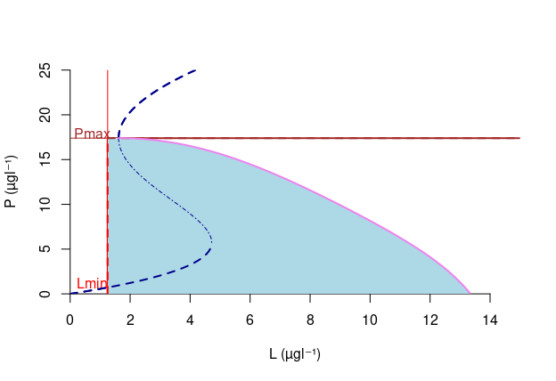
Next figure shows the result for the following parameters:  $b=1.95$ an$^{-1}$ ; $q=1.9$ ; $m=19.44\  \mu gl^{-1}$; $r=72.22\  \mu gl^{-1}$ an$^{-1}$; $L_{min}=1.25\  \mu gl^{-1}$ ; $P_{max}=17.39\  \mu gl^{-1}$ ;   $|u_{min}|=u_{max}=3.15$.

Because the boundary of this viability problem can be described using an integral curve, it is possible to assess the accuracy of approximations generated by generic software.

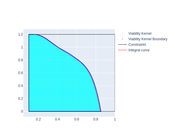
Shown below the comparison for $b=0.8$ year$^{-1}$ ; $q=8$ ; $m=1\  \mu gl^{-1}$; $r=1\  \mu gl^{-1}$ year$^{-1}$; $L_{min}=0.1\  \mu gl^{-1}$ ; $P_{max}=1.2\  \mu gl^{-1}$ ;   $-u_{min}=u_{max}=0.09$ between the viability kernel defined by the integral curve (in red) and the approximate result obtained using the ViabLab software on a regular 3001×3001 grid (light blue set with a dark blue boundary):

 It can be seen that the kernel approximation is well performed from the outside.