LUNDI 27 avril
LUNDI 27 AVRIL
8h15 - Rendez-vous de l’ensemble des participants devant la Bibliothèque Universitaire
SESSION 1 : POSER UN PROBLEME EN VIABILITE
Animateur : Bates – De Lapparent - Lavallée - Désilles
8h30 - 8h50 La viabilité mathématique en question ? (Samuel Bates)
8h50 - 9h50 Concept et illustration du noyau de viabilité (François Lavallée)
Pause & discussion
10h00-11h15 Formuler mathématiquement un problème de viabilité (François Lavallée)
11h15-12h00 Cas de résolution analytique de la viabilité (François Lavallée)
Déjeuner
13h30-14h15 Cas de résolution numérique de la viabilité (François Lavallée)
14h15-15h00 Cas de résolution de viabilité avec cible terminale (François Lavallée)
Pause & discussion
15h15-16h00 Cas de résolution de viabilité en situation de risque (François Lavallée)
16h00-16h45 Cas de résolution de viabilité en situation d’incertitude (François Lavallée)
Pause & discussion
17h00-17h45 Cas de résolution de viabilité multi-agent (Alice De Lapparent)
MARDI 28 AVRIL
SESSION 2 : L’INFORMATIQUE DE LA VIABILITE
Animateur : Désilles - Lavallée
8h00-9h00 Préparation à l’informatique de la viabilité (Anya Désilles)
9h00-10h30 Présentation du logiciel Viablab (Anya Désilles)
Pause & discussion
10h45-11h15 Enjeux informatiques sur les noyaux de viabilité (Anya Désilles)
11h15-12h00 Enjeux informatiques sur les trajectoires de viabilité (Anya Désilles)
Déjeuner
13h30-15h30 Atelier de manipulation du Logiciel autour d’un cas d’étude (1/2) (François Lavallée & Anya Désilles)
Pause & discussion
15h45-17h45 Atelier de manipulation du Logiciel autour d’un cas d’étude (2/2) (François Lavallée & Anya Désilles)
MERCREDI 29 AVRIL
SESSION 3 : ATELIERS THEMATIQUES D’APPLICATION
Animateurs Désilles - Gloglo
8h00-10h00 Atelier autour de AgroViablab : Illustration vers une montée en
complexité (Anya Désilles)
Pause & discussion
10h15-12h15 Brainstorming autour d’AgroViablab (collectif)
Déjeuner
13h45-15h45 Atelier d’application sur un système monétaire : Illustration vers une simplification de complexité (Beringer Gloglo)
15h45-17h45 Brainstorming sur les applications (collectif)
18h00-19h00 Séminaire sur la viabilité en économie monétaire (en marge de l’école chercheur à destination des étudiants de Master d’économie) (Beringer Gloglo, Samuel Bates)
JEUDI 30 AVRIL
SESSION 4 : MODELISATION EN VIABILITE
8h00-09h00 Brainstroming autour d’un 1er sujet de modélisation (collectif)
9h00-10h00 Brainstroming autour d’un 2e sujet de modélisation (collectif)
Pause & discussion
10h15-11h15 Brainstroming autour d’un 3e sujet de modélisation (collectif)
11h15-12h00 Retour d’expériences
Déjeuner & clôture hors les murs (13h00-17h00 : Saint-Pierre)
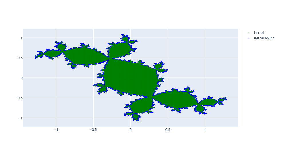
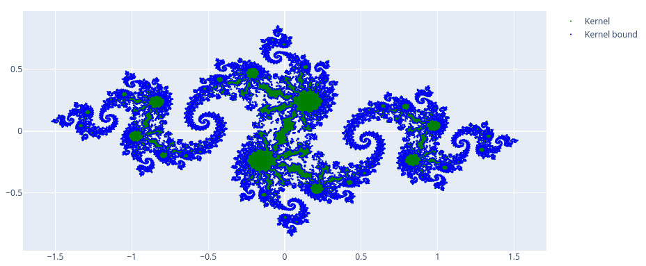
To compute apporximations of these viability kernels, simply place the .cpp file in ViabLab's /source directory and the .json file in the /INPUT directory.
Then, run ViabLab ; the output files will be placed in the /OUTPUT directory.
To visualize the viability kernel and its boundary, place the .py file in the /OUTPUT directory and run it.
For assistance, consult the training materials.