Mathématique

Dans le cas où f $\phi$ est un polynôme, l'ensemble de Julia rempli est le complémentaire du bassin d'attraction du point à l'infini; autrement dit, ce sont les points dont l'orbite est bornée. 

Étant donnés un nombres complexes, $u:=a+ib$, soit la fonction complexe $\phi(z)=z^2+c$ ou de manière équivalente, la fonction $\phi(x,y):=(x^2-y^2+a,2xy+b)$ avec $z=x+iy$, on considère la suite $(z_n)$ définie par la relation de récurrence : $z_{n+1}=\phi(z_n,u)$ avec $\phi(z)=z^2+c$,

Pour une valeur donnée de $u$, l'ensemble de Julia correspondant est la frontière de l'ensemble des valeurs initiales $z_0$ pour lesquelles la suite est bornée. 

D'après

Aubin, J.-P., Bayen, A., & Saint-Pierre, P. Viability Theory: New Directions. Springer. 2011.

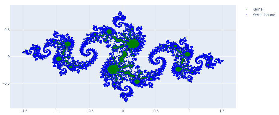
Le sous-ensemble $K_u:=Viab_{\phi}(B(0,1))$ est le sous-ensemble de Julia rempli pour la function $\phi$ et sa frontière $J_u:=\partial K_u$ est l'ensemble de Julia.

L'Algorithme de Viabilité permet donc de calculer une approximation de ces ensembles de Julia.

Voici le noyau de viabilité approché obtenu en utilisant le logiciel VIABLAB : 

Pour calculer ce noyau de viabilité avec VIABLAB, utilisez les deux fichiers ci-dessous en suivant cette procédure :

Introduction

Le problème d'eutrophisation du lac décrit comme le problème de viabilité du lac et des exploitations riveraines est traité à un niveau global et suppose un décideur unique. Dans le présent exemple les parties prenantes sont réunies dans un comité, et les membres du comité (appelés individus dans la suite) ne sont pas nécessairement d'accord sur la dynamique du lac. Cet exemple illustre les cas où la gestion est collective et où il n'y a pas de consensus sur la dynamique. Ce problème est un problème de viabilité garantie.

Ce problème est décrit en détail dans :

Alvarez, I., Zaleski, L., Briot, J.-P., Irving, M. de A. (2023). Collective management of environmental commons with multiple usages: A guaranteed viability approach. Ecological Modelling, 475, Article 110186

Version auteur disponible ici

Les caractéristiques 

Les caractéristiques du problème modélisé sont les suivantes :  

1.  $N$ individus utilisent les même variables pour décrire le système. Dans cet exemple du lac, ce sont les mêmes variables $L$ (apports de phosphore) et $P$ (concentration totale de phosphore) que dans le cas du décideur unique.
2. Les contrôles admissibles retenus dans les modèles sont communs à tous les individus. On garde donc la même variable de contrôle et les mêmes bornes : $u\in U=[u_{min},u_{max}]$.
3. Tous les individus $i$ peuvent définir un ensemble d'états souhaitables $K_i$ dont l'intersection est non vide. On garde donc un ensemble de contraintes similaires au cas du décideur unique :  $x=\left(L(t),P(t)\right) \in K=[L_{min}, +\infty[ \times [0,P_{max}]$
4. La dynamique du système est modélisée pour chaque individu par un ensemble d'équations (ou d'inclusion différentielles) $S_i$
5. L'objectif de chaque individu est de maintenir le système modélisé par leur dynamique $S_i$ dans leur ensemble d'états souhaitables $K_i$

6. Les individus acceptent de partager leurs informations personnelles avec un tiers de confiance.

   Dans cet exemple, on considère $N=4$ individus. Trois d'entre eux ($i\in\{1,2,3\}$) adoptent la dynamique classique, mais avec des paramètres différents :

   \begin{equation} 
   (P_i \text{ modèle 1})\left\{
   \begin{array}{l}
   \frac{dL}{dt}=u\in U=\left[ u_{min},u_{max}\right] \\
   \frac{dP}{dt}=-b_i P(t) + L(t) +r_i\frac{P(t)^{q_i}}{m_i^{q_i} + P(t)^{q_i}} \\
   \left(L(t),P(t)\right) \in K=[L_{min}, +\infty[ \times [0,P_{max}]
   \end{array}
   \right.
   \end{equation}

   Un individu ($i=4$) considère que le processus de relargage peut se produire différemment, et utilise une formule différente pour la pseudo-sygmoïde :

   \begin{equation}
   (S' \text{ modèle 0}) \quad \frac{dP}{dt}=-b_i P(t) + L(t) + r_i \frac{P(t)}{P(t) + m_i e^{(-\lambda_i(P(t)-m_i)) }}
   \end{equation}

   Les valeurs numériques pour les calculs sont les suivantes : $u_{min}=-u_{max}/2$ ; $u_{max}\approx 3,15\; \mu g.l^{-1}.\text{an}^{-1}$, $L_{min}\approx6,94 \; \mu g.l^{-1}$,  $P_{max}=24.76 \; \mu g.l^{-1}$, 

Le  tableau suivant rassemble les valeurs des paramètres pour chaque individu (b,r,m sont en $\mu g.l^{-1}$).

Les incertitudes sont traitées comme des variables prenant leur valeur dans des ensembles. Le problème est un problème de viabilité garantie, dans lequel le vecteur $v$ des "tyches" regroupent les paramètres incertains : $v_1$ représente le paramètre $b_i$, $v_2$ : $\alpha_i$, $v_3$ : $q_i$ et $v_4$ représente $\lambda_i$. La dynamique du modèle avec incertitudes devient :

\begin{equation}
f_v(x=(L,P),u,v)=\left( 
\begin{array}{l}
u\\
- v_1 P + L +  r \left( (1-v_2) \frac{P^{v_3}}{m^{v_3} + P^{v_3}} + v_2 \frac{P}{P + m e^{(-v_4(P-m)) }}\right)  \;
\end{array}
\right)
\end{equation}

Problèmes

Le problème de viabilité garantie qui doit être résolu est le suivant :

\begin{equation}
(P_v)\left\{
\begin{array}{lcl}
(L,P)'(t)&=&f_B((L,P)(t),u(t),v(t))\\
u(t)&\in& U=\left[ u_{min},u_{max}\right] \\
v(t)&\in & V=[2.2,2.3]\times[0,1]\times[2.2,2.3]\times[1/19,1/18]\\
(L,P)(t) &\in& K \; 
\end{array}
\right.
\end{equation}

Le noyau garanti peut être approximé avec ViabLab (version 2.2). Le code correspondant est ici : https://forge.inrae.fr/isabelle.alvarez/emlake

Introduction 

L'accumulation de nutriments (comme le phosphore ou l'azote) dans l'eau d'un lac peut amener un changement d'état qui s'accompagne de prolifération d'algues, de dégradation de la qualité de l'eau et de la biodiversité, éventuellement de bloom bactérien : c'est l'eutrophisation. Le problème du lac et des exploitations riveraines consiste à   déterminer s'il est possible de concilier la pratique d'une activité qui apporte des nutriments et la conservation du lac dans un état souhaitable (oligotrophe, par opposition à eutrophe).

Ce problème est décrit en détail dans :

S. Martin. The cost of restoration as a way of defining resilience: a viability approach applied to a model of lake eutrophication. Ecol. Soc.   http://www.ecologyandsociety.org/vol9/iss2/art8

On souhaite que les apports $L$L soient supérieurs à un seuil $L_{min}$Lmin, pour tenir compte des besoins de l'activité des exploitations riveraines ; et que la concentration du phosphore total, $P$, P soit inférieure à un seuil Pmax $P_{max}$ pour conserver le lac oligotrophe. Ces états souhaitables constituent l'ensemble de contraintes $K=[L_{min}, +\infty[ \times [0,P_{max}]$.

L'évolution de la concentration du phosphore total dans le lac est modélisée par une pseudo-sygmoïde :

$$\frac {dP} {dt}=-bP(t)+L(t)+r\frac {P(t)^{q}} {m^{q} + P(t)^{q}} \qquad$$

On suppose que l'évolution des apports de phosphore peut être contrôlée (par des unités de dépollution, la mise en place de zones humides, le changement de pratique agricoles ou industrielles, etc.) et on modélise ces contrôles par une grandeur unique $u\in U=[u_min,u_max]$u∈U=[umin,umax]. La dynamique des apports est modélisée par :

$$\frac {dL} {dt}=u \in [- u_{min}, u_{max}] \qquad$$

Le problème de viabilité est donc défini par :

\begin{equation}
(P)\left\{
\begin{array}{l}
\frac{dL}{dt}=u\in U=\left[ u_{min},u_{max}\right] \\
\frac{dP}{dt}=-b P(t) + L(t) +r\frac{P(t)^{q}}{m^{q} + P(t)^{q}} \\
\left(L(t),P(t)\right) \in K=[L_{min}, +\infty[ \times [0,P_{max}]
\end{array}
\right.
\end{equation}
 

Exemple 1

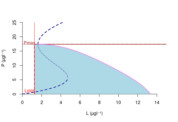
Le noyau de viabilité peut être obtenu par le calcul d'une courbe intégrale (voir page 7 dans https://arxiv.org/pdf/2107.02684 ). La figure suivante montre le résultat pour les paramètres suivants : $b=1,95$ an$^{-1}$ ; $q=1,9$ ; $m=19,44\  \mu gl^{-1}$; $r=72,22\  \mu gl^{-1}$ an$^{-1}$; $L_{min}=1,25\  \mu gl^{-1}$ ; $P_{max}=17,39\  \mu gl^{-1}$ ;   $|u_{min}|=u_{max}=3,15$.

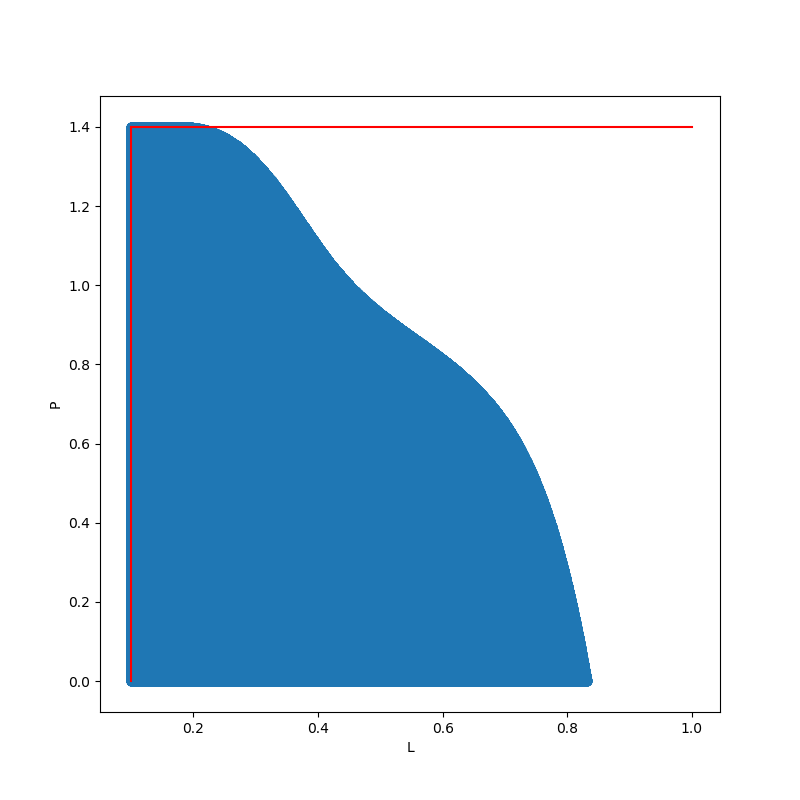
Une approximation peut être calculée directement avec des logiciels de calcul de noyau comme ViabLab.

Pour la release 1 de ViabLab, voici les codes utilisés correspondants à l'exemple développé ci-dessus.

Fichier .json (à placer dans le répertoire: VIABLAB/INPUT): Lac_params.json

Fichier .h (à placer dans le répertoire:: VIABLAB/source/data : data_Lac.h

Ces fichiers correspondent aux paramètres suivants : $b=0.8$ year$^{-1}$ ; $q=8$ ; $m=1\  \mu gl^{-1}$; $r=1\  \mu gl^{-1}$ year$^{-1}$; $L_{min}=0.1\  \mu gl^{-1}$ ; $P_{max}=1.4\  \mu gl^{-1}$ ;   $|u_{min}|=u_{max}=0.09$.

Le contrôle est discrétisé sur 3 valeurs étant donné les spécificités du problème.

La discrétisation est faite sur 5000 points / axe. L'approximation calculée par ViabLab est montrée sur la figure suivante. En rouge les seuils des contraintes. On voit que l'approximation du noyau est bien faite par l'extérieur.