Beginner

Language diversity

Niveau de difficulté
Mathematical framework
Continuous time
Continuous space
Viability kernel
Contenu

Introduction

Many languages ​​are at risk of disappearing. It is therefore crucial to understand the mechanisms underlying changes in the number of speakers and to determine if there are measures that could help preserve some of them.

In their article,

Abrams, S. Strogatz, Modelling the dynamics of language death, Nature 424 (6951) (2003) 900

Abrams and Strogatz proposed a mathematical model for studying language competition.

This model fits well with several sets of empirical data: it satisfactorily accounts for historical data concerning the decline of Welsh, Scottish Gaelic, Quechua, and other endangered languages.

In the Abrams and Strogatz model, as well as in those derived from it, the population size is assumed to remain constant. Therefore, the variables are the proportions of the different speaker groups. In models that include bilingualism, the population consists of three groups: monolingual speakers of language A, monolingual speakers of language B, and bilingual speakers AB. The model is two-dimensional, with $\sigma_A$ representing the proportion of speakers of language A and $\sigma_B$ the proportion of speakers of language B ($\sigma_{AB} = 1 - \sigma_A - \sigma_B$).

Within any linguistic subpopulation, forces and influences lead members of one group to switch languages ​​in favor of another. In the Abrams and Strogatz model, the rate at which speakers of one language learn the second language depends on the attractiveness of the latter. In their most general definition of attractiveness, Abrams and Strogatz postulate that a language is more attractive the more speakers it has and the higher its prestige.

In their article,

C. Bernard, S. Martin, Building strategies to ensure language coexistence in presence of bilingualism, Appl. Math. Comput. (2012), doi:10.1016/j.amc.2012.02.041

The authors model only the transitions of the following four types: A → AB, AB → A, A → AB, and AB → B (with the transitions A → B and B → A being extremely rare in practice). They also assume an asymmetry between monolinguals and bilinguals: A → AB (or B → AB) occurs at a rate proportional to the attractiveness of monolingual speakers of A (or B); AB → A (or AB → B) occurs at a rate proportional to the attractiveness of the entire pool of speakers of A, including bilinguals (thus, some bilinguals can become monolingual speakers of A even if A has no monolingual speakers).
Consequently, the two-dimensional model is defined by:

$$
\left\{\begin{array}{ll}
\sigma_A' &= (1-\sigma_A-\sigma_B)(1-\sigma_B)^as_A-\sigma_A\sigma_B^as_B\\
\sigma_B' &= (1-\sigma_A-\sigma_B)(1-\sigma_A)^as_B-\sigma_B\sigma_A^as_A
\end{array}\right.
$$

where $s_A$ (resp. $s_B$) denotes the prestige of language A (resp. B), and $a$ is a parameter modeling how the attractiveness of a language varies with the proportion of its speakers.
For convenience, the authors assume that $s_A+s_B=1$, allowing the substitutions $s_A=s$ and $s_B=1-s$.

The problem of the coexistence of two languages

Bernard and Martin consider that prestige, $s$, can evolve (under the influence of public action, for example), but that its variation at each time step is limited. Thus,

$$
s' = u\in U=[\underline{u};\bar{u}]
$$

When $u>0$, the prestige of language A increases and that of B decreases; the reverse occurs when $u<0$.

The dynamics of the system are thus described by:

$$
\left\{\begin{array}{ll}
\sigma_A' &= (1-\sigma_A-\sigma_B)(1-\sigma_B)^as-\sigma_A\sigma_B^a(1-s)\\
\sigma_B' &= (1-\sigma_A-\sigma_B)(1-\sigma_A)^a(1-s)-\sigma_B\sigma_A^as\\
s' &= u\in U=[\underline{u};\bar{u}]
\end{array}\right.
$$

The authors propose seeking strategies based on prestige variations that ensure the coexistence of the two languages—that is, strategies that maintain a certain level of monolingual speakers for each language. The set of constraints can thus be written as follows:

$$
K:= [\underline{\sigma};1]\times[\underline{\sigma};1]\times [0;1]
$$

Solving this problem means finding the set of states $(\sigma_A, \sigma_B, s)$ from which it is possible to maintain a certain proportion of monolingual groups by manipulating the relative prestige of the two languages—that is, the viability kernel in the terminology of viability theory.


Dynamics Controls Uncertainties Constraints Target Viability Concept

Continuous time

Continuous 3-dimensional space

$
\left\{\begin{array}{ll}
\sigma_A' &= (1-\sigma_A-\sigma_B)(1-\sigma_B)^as-\sigma_A\sigma_B^a(1-s)\\
\sigma_B' &= (1-\sigma_A-\sigma_B)(1-\sigma_A)^a(1-s)-\sigma_B\sigma_A^as\\
s' &= u
\end{array}\right.
$

$(\sigma_A,\sigma_B,s)\in [0;1]\times[0;1]\times [0;1]\cap \{\sigma_A+\sigma_B\leq 1\}
$

Parameter : $a$

$u\in U=[\underline{u};\bar{u}]$

Parameters : $\underline{u},\bar{u}$

None

$
K:= [\underline{\sigma};1]\times[\underline{\sigma};1]\times [0;1]
$


Parameters : $\underline{\sigma}$

None Viability kernel

Results

In the article cited above, the authors provided an analytical description of the viability kernel boundary, composed of integral curves originating from specific points on the boundary of the constraint set.
To illustrate their result, they reproduced the viability kernel for the parameter values ​​$a=1.41$, $\underline{u}=-0.06$, $\bar{u}=0.06$, and $\underline{\sigma}=0.1$.

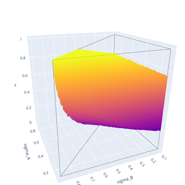
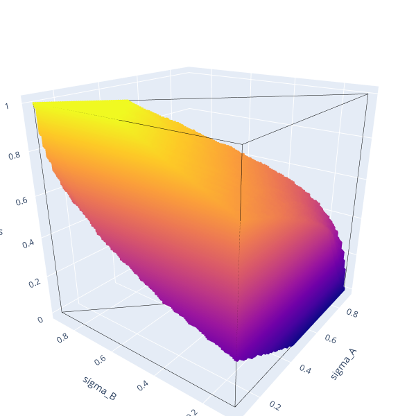
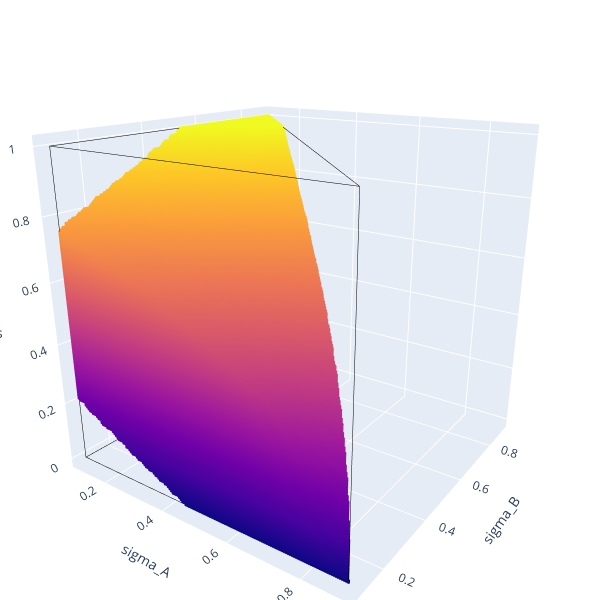
Below, we present four 3D views of the viability kernel approximation corresponding to these parameter values, generated using the ViabLab software based on a $201 \times 201 \times 201$ grid of points (the black lines represent the edges of the constraint set):
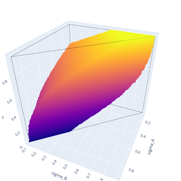
As expected, the kernel is invariant under the transformation $\sigma_A\rightarrow \sigma_B$, $\sigma_B\rightarrow \sigma_A$, and $s\rightarrow 1-s$.

Non-viable situations correspond to states from which:

  • even a continuous increase in the prestige of language A—at maximum intensity—up to its maximum value of 1 would not prevent the proportion of its speakers from crossing the threshold $\underline{\sigma}$,
  • or even a continuous increase in the prestige of language B—at maximum intensity—up to its maximum value of 1 would not prevent the proportion of its speakers from crossing the threshold $\underline{\sigma}$.
Commentaires

We provide the files needed to calculate the aforementioned approximations using the ViabLab software below.

Please consult the training materials:

  • to perform the calculation
  • to understand and visualize the results.

Grazing management - shoot and crown biomass

Niveau de difficulté
Domain
Mathematical framework
Continuous space
Viability kernel
Continuous time
Contenu

Introduction

A major challenge in managing grazed pastures lies in reconciling conflicting objectives: increasing short-term profits while preserving the long-term viability of the rangeland. Increasing the stocking rate (number of animals per hectare) boosts short-term returns but can lead to virtually irreversible environmental degradation if the resulting grazing pressure is excessive. Conversely, maintaining an excessively low stocking rate can result in significant lost revenue.

In the article

Anderies, J., Janssen, M. & Walker, B. Grazing Management, Resilience, and the Dynamics of a Fire-driven Rangeland System. Ecosystems 5, 23–44 (2002). https://doi.org/10.1007/s10021-001-0053-9

The authors use the following model to account for the interactions between grass growth and grazing pressure:

$$
\left\{\begin{array}{ll}
c' &= r_cs-\delta_cc\\
s'&= c(a_c+r_ss)(1-\frac{s}{s^*}-\alpha_{ws}(\frac{w}{w^*})^\beta)-\gamma_gs\\
w'&=r_ww(1-\frac{w}{w^*})
\end{array}\right.
$$

Regarding the grass, $c(t)$ and $s(t)$ represent the biomass of the crown (roots plus growing points) and the shoot part, respectively, at time $t$. The parameter $s^*$ corresponds to the maximum shoot biomass per unit area, while $\gamma_g\leq 1$ represents the fraction of the shoot part removed by the grazing pressure exerted by the animals present. The crown grows at a rate $r_cs$ in the presence of shoot parts and declines at a rate $\delta_c$.
$a_c$ corresponds to the growth rate of shoot biomass per unit of crown biomass, and $r_s$ to the growth rate of shoot biomass per unit of crown biomass and per unit of shoot biomass.

Grass growth is also affected by the presence of shrubs: $w(t)$ represents shrub biomass, $r_w$ the intrinsic growth rate of shrubs, $w^*$ the maximum shrub biomass per unit area, and $w_s (=w/w^*)$ models the competitive effect of shrubs on the grass. The parameter $\beta$ measures the relative non-linearity of this effect.

The pasture manager's viability problem

The objective of rangeland management is to identify intervention strategies (adjustments to stocking rates) that reconcile two constraints: providing sufficient feed for the animals while preserving grass quality.

In the article

Martin S. Viability analysis as an approach for assessing the resilience of agroecosystems. In: Gardner SM, Ramsden SJ, Hails RS, eds. Agricultural Resilience: Perspectives from Ecology and Economics. Ecological Reviews. Cambridge University Press; 2019:273-294.

The authors study this viability problem using a simplified grass growth model, assuming that the maximum shoot biomass value, $s^*$, is 1 and that the impact of the shrub population is negligible—that is: 

$$
s^* = 1 \text{ et } \alpha_{ws} = 0.$$

The possible intervention on the system involves varying the grazing pressure—a variation assumed to be bounded—since purchasing or selling animals takes time :

$$
\gamma'(t) = u(t) \in [u_{min},u_{max}].
$$

The dynamics of the system are thus described by:

$$
\left\{\begin{array}{ll}
c' &= r_cs-\delta_cc\\
s'&= \frac{r_c}{\delta_c}s(a_c+r_ss)(1-s)-\gamma_gs\\
\gamma_g'&= u \in [u_{min},u_{max}]
\end{array}\right.
$$

The constraint regarding grass quality is modeled by a shoot biomass value exceeding a threshold, $s_{min}$, to ensure regrowth. The constraint regarding livestock feed is modeled by a grazing pressure that also exceeds a threshold, $\underline{g}$, over time. The set of constraints can thus be written as:

$$
K(s_{min},\underline{g}):=R^+\times [s_{min},+\infty[\times  [\underline{g},1]
$$

Solving this problem means finding the set of states $(s, \gamma_g)$ from which it is possible to feed the herd while maintaining high-quality grass by adjusting the number of animals—in other words, the viability kernel within the framework of viability theory.


Dynamiques Controls Uncertainties Constraints Target Viability concept

Continuous time

Continuous 3-dimensional space

$
\left\{\begin{array}{ll}
c' &= r_cs-\delta_cc\\
s'&= \frac{r_c}{\delta_c}s(a_c+r_ss)(1-s)-\gamma_gs\\
\gamma_g'&= u 
\end{array}\right.
$

Parameters : $r_c, \delta_c, a_c, r_s$

$u\in U=\left[ u_{min},u_{max}\right]$

Parameters : $u_{min},u_{max}$

None

$
K(s_{min},\underline{g}):=R^+\times [s_{min},+\infty[\times  [\underline{g},1]
$


Parameters : $s_{min},\underline{g}$

None Viability kernel

Résultats

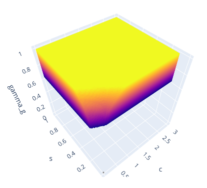
In the article cited above, the parameter values ​​are as follows: $r_c=1$, $\delta_c=1$, $a_c=0.1$,  $r_s=3$,  $s^*=1$, $u_{min} = -0.05$, $u_{max} = 0.05$, $s_{min} = 0.1$, $\underline{g}=0.65$.

We reproduce below the approximation of the viability kernel associated with these parameter values, generated by the ViabLab software using a 201×201×201 point grid:


View of the 3D viability kernel approximation.


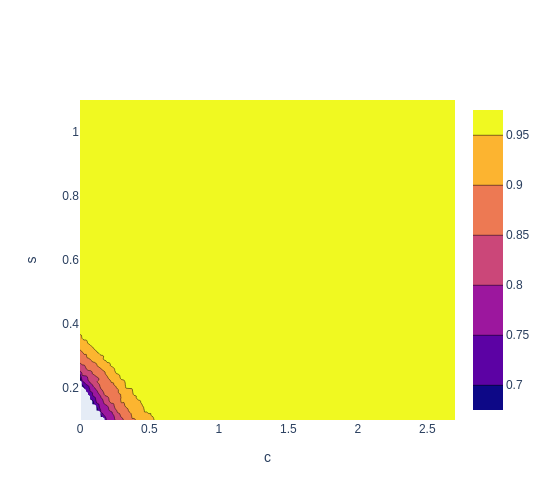
Maximum grazing pressure value that remains viable for the various stem and crown biomass values: $\max_{(c,s,\gamma_g)\in Viab(K)}\gamma_g$.


As expected, starting from a higher grazing pressure results in a more restricted set of shoot and crown biomass combinations for which the system is viable.

This restriction is more pronounced when the capacity to reduce this pressure is low—that is, when $u_{min}$ approaches 0.


Commentaires

We provide the files needed to calculate the aforementioned approximations using the ViabLab software below.

Please consult the training materials:

  • to perform the calculation
  • to understand and visualize the results.

Grazing management - shoot biomass

Niveau de difficulté
Domain
Mathematical framework
Continuous space
Viability kernel
Continuous time
Contenu

Introduction

A major challenge in managing grazed pastures lies in reconciling conflicting objectives: increasing short-term profits while preserving the long-term viability of the rangeland. Increasing the stocking rate (number of animals per hectare) boosts short-term returns but can lead to virtually irreversible environmental degradation if the resulting grazing pressure is excessive. Conversely, maintaining an excessively low stocking rate can result in significant lost revenue.

In the article

Anderies, J., Janssen, M. & Walker, B. Grazing Management, Resilience, and the Dynamics of a Fire-driven Rangeland System. Ecosystems 5, 23–44 (2002). https://doi.org/10.1007/s10021-001-0053-9

The authors use the following model to account for the interactions between grass growth and grazing pressure:

$$
\left\{\begin{array}{ll}
c' &= r_cs-\delta_cc\\
s'&= c(a_c+r_ss)(1-\frac{s}{s^*}-\alpha_{ws}(\frac{w}{w^*})^\beta)-\gamma_gs\\
w'&=r_ww(1-\frac{w}{w^*})
\end{array}\right.
$$

Regarding the grass, $c(t)$ and $s(t)$ represent the biomass of the crown (roots plus growing points) and the shoot part, respectively, at time $t$. The parameter $s^*$ corresponds to the maximum shoot biomass per unit area, while $\gamma_g\leq 1$ represents the fraction of the shoot part removed by the grazing pressure exerted by the animals present. The crown grows at a rate $r_cs$ in the presence of shoot parts and declines at a rate $\delta_c$.
$a_c$ corresponds to the growth rate of shoot biomass per unit of crown biomass, and $r_s$ to the growth rate of shoot biomass per unit of crown biomass and per unit of shoot biomass.

Grass growth is also affected by the presence of shrubs: $w(t)$ represents shrub biomass, $r_w$ the intrinsic growth rate of shrubs, $w^*$ the maximum shrub biomass per unit area, and $w_s (=w/w^*)$ models the competitive effect of shrubs on the grass. The parameter $\beta$ measures the relative non-linearity of this effect.

The pasture manager's viability problem

The objective of rangeland management is to identify intervention strategies (adjustments to stocking rates) that reconcile two constraints: providing sufficient feed for the animals while preserving grass quality.

In the article

Martin, Sophie & Deffuant, Guillaume & Calabrese, Justin. (2011). Defining Resilience Mathematically: From Attractors To Viability. 10.1007/978-3-642-20423-4_2. 

the authors study this viability problem using a simplified grass growth model, assuming that the shrub population remains constant at its equilibrium value and that the crown biomass instantly reaches the equilibrium value associated with the shoot biomass:

$$
w = w^* \text{ and  } c = \frac{r_c}{\delta_c}s.
$$

The possible intervention on the system involves varying the grazing pressure—a variation assumed to be bounded—since purchasing or selling animals takes time :

$$
\gamma'(t) = u(t) \in [u_{min},u_{max}].
$$

The dynamics of the system are thus described by:

$$
\left\{\begin{array}{ll}
\gamma_g'&= u \in [u_{min},u_{max}]\\
s'&= \frac{r_c}{\delta_c}s(a_c+r_ss)(1-\frac{s}{s^*}-\alpha_{ws})-\gamma_gs.
\end{array}\right.
$$

The constraint regarding grass quality is modeled by a shoot biomass value falling between two limits: a lower limit to ensure regeneration and an upper limit to preserve nutritional quality. The constraint regarding livestock feed is modeled by a grazing pressure that must also remain above a certain threshold over time. The set of constraints can thus be expressed as follows:

$$
K(\underline{g},s_{min},s_{max}):=[\underline{g},1]\times [s_{min},s_{max}].
$$

Solving this problem means finding the set of states $(s, \gamma_g)$ from which it is possible to feed the herd while maintaining high-quality grass by adjusting the number of animals—in other words, the viability kernel within the framework of viability theory.

Dynamics Controls Uncertainties Constraints Target Viability Concept

Continuous time

Continuous 2-dimensional space

\begin{equation}
\left\{\begin{array}{ll}
\gamma_g'&= u\\
s'&= \frac{r_c}{\delta_c}s(a_c+r_ss)(1-\frac{s}{s^*}-\alpha_{ws})-\gamma_gs\\ 
\end{array}\right.
\end{equation}

Paramaters : $r_c, \delta_c, a_c, r_s, s^*,  \alpha_{ws}$

$u\in U=\left[ u_{min},u_{max}\right]$

Parameters : $u_{min},u_{max}$

Aucune

$
K(\underline{g},s_{min},s_{max}):=[\underline{g},1]\times [s_{min},s_{max}].
$


Parameters : $\underline{g}, s_{min},s_{max}$

None Viability kernel

Results

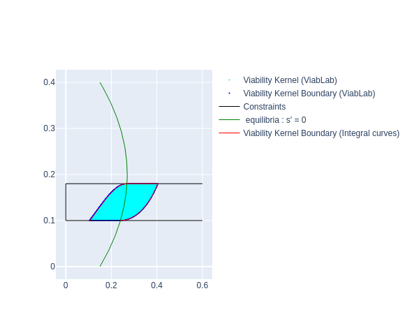
For the parameter values ​​from the article cited above ($r_c=1$, $\delta_c=1$, $a_c=0.3$, $r_s=3$, $s^*=1$, $\alpha_{ws}=0.5$, $u_{min} = -0.02$, $u_{max} = 0.02$, $\underline{g}=0$, $s_{min} = 0.1$, $s_{max} = 0.18$), the viability kernel can be obtained by calculating two integral curves (the authors of the article did not elaborate on this point).

Indeed, its boundary is defined by a closed curve formed by subsets of the boundary of the constraint set $K$ and two integral curves:

  • the one originating from the point $(\gamma_g^1,s_{min}) $ with $s'(\gamma_g^1,s_{min})) = 0$ that follows the backward dynamics: 
    \begin{equation}
    \left\{\begin{array}{ll}
    \gamma_g'&= -u_{min}\\
    s'&= -(\frac{r_c}{\delta_c}s(a_c+r_ss)(1-\frac{s}{s^*}-\alpha_{ws})-\gamma_gs)\\ 
    \end{array}\right.
    \end{equation}
  • the other originating from the point $(\gamma_g^2,s_{max}) $ with $s'(\gamma_g^2,s_{max})) = 0$ that follows that follows the backward dynamics: 
    \begin{equation}
    \left\{\begin{array}{ll}
    \gamma_g'&= -u_{max}\\
    s'&= -(\frac{r_c}{\delta_c}s(a_c+r_ss)(1-\frac{s}{s^*}-\alpha_{ws})-\gamma_gs)\\ 
    \end{array}\right.
    \end{equation}

The following figure shows the boundary of the viability kernel as a closed curve, along with the approximation obtained using the ViabLab software on a 2001 × 2001 grid of points. The result is consistent with the graph in the original article and is far more precise in the section of the kernel boundary that coincides with the boundary of the constraint set, as well as in the section defined by the integral curves.

Commentaires

We provide the files needed to calculate the aforementioned approximations using the ViabLab software below.

Please consult the training materials:

  • to perform the calculation
  • to understand and visualize the results.

Toy exemple : a disk inside a square

Niveau de difficulté
Domain
Mathematical framework
Viability kernel
Contenu

Here is an example where we know the viability kernel.

Indeed, let's consider two-dimensional dynamics where the orbit of the points on the circle centered at the origin of the coordinate system and with radius $a$ is the same circle; where the orbit of the points with a norm strictly less than $a$ is a spiral tending towards the origin, and where the orbit of the points with a norm strictly greater than $a$ is a spiral which diverges.

This is the case for the solutions of the equation $x'=f(x)$ with

$$
f(x_1,x_2):=(\frac{||x||-a}{||x||}x_1+x_2 ; -x_1+\frac{||x||-a}{||x||}x_2)
$$   

Let us consider a square as a constraint set  : 

$$
K := \{(x_1,x_2)\in R^2\,|\, |x_1|\leq c \text{ et } |x_2|\leq c \}.
$$

Clearly, the set of points from which trajectories originate that remain within $K$ indefinitely is the disk centered at the origin with radius $a$.

This example makes it possible to test the precision of approximations obtained using generic software.

Dynamics Controls Uncertainties Constraint Target Viability concept

Continuous time

2-dimensional continuous space

$f(x_1,x_2):=(\frac{||x||-a}{||x||}x_1+x_2 ; -x_1+\frac{||x||-a}{||x||}x_2)
$

Parameter : $a$

None None

$\{(x_1,x_2)\in R^2\,|\, |x_1|\leq c \text{ et } |x_2|\leq c \}$


Parameter : $c$

None Viability kernel

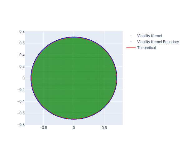
Below is a comparison, for $a = 0.7$ and $c=1.5$, between the theoretical result (the disk bounded by the red circle) and the approximate result obtained using the ViabLab software on a regular 2001×2001 grid (the green set bounded by the blue line):


Commentaires

We provide the files needed to calculate the aforementioned approximations using the ViabLab software below.

Please consult the training materials:

  • to perform the calculation
  • to understand and visualize the results.
Fichier(s) de code

[Texte] Fichiers de sortie de ViabLab en anglais

Niveau de difficulté
Thématique
Présentation formation

Les fichiers de sortie de ViabLab

Les fichiers sorties de ViabLab se trouvent dans le répertoire ~/ViabLabGui/bin/VIABLAB/OUTPUT.

Un calcul génère plusieurs fichiers qui sont nommés avec le même préfixe.

Le fichier <prefixe>-grid_data.dat contient les informations sur le grille régulière sur laquelle est basée le calcul, ci-dessous un exemple :

2  ---- nombre de dimensions de l'espace des états
-2 ---- première coordonnée du point inférieur (dans toutes les dimensions) de la grille 
-2 ---- deuxième (ici seconde puisqu'on est en dimension 2) coordonnée du point inférieur (dans toutes les dimensions) de la grille
2  ---- première coordonnée du point supérieur (dans toutes les dimensions) de la grille
2  ---- deuxième (ici seconde puisqu'on est en dimension 2) coordonnée du point inférieur (dans toutes les dimensions) de la grille
4001 -- nombre de points de la grille selon le premier axe
4001 -- nombre de points de la grille selon le second axe
0
0     Anya HELP !
1
1

Le fichier <prefixe>-viab.dat contient les coordonnées des points de la grille suivies de 0.0 si le point n'appartient pas au noyau calculé et 1.0 s'il y appartient ; le nombre de colonnes est donc égale au nombre de dimensions de l'espace des états plus 1.

Le fichier <prefixe>-viab-bound.dat contient la liste des coordonnées des points de la grille qui ont au moins un voisin qui n'appartient pas au noyau calculé. Ils représentant la frontière de ce noyau.

[Texte] ViabLab installation from GitHub

Niveau de difficulté
Thématique
Présentation formation

How to install and compile ViabLab from GitHub

Contenu
MAC OS
Read more 

Step 1. Copy VIABLAB from GitHub 

Go to https://github.com/lastre-viab/VIABLAB, click on Code button and download the ZIP file VIABLAB-main.zip. 

Open Finder, create the folder viablab that will contain the  program and results and unzip VIABLAB-main.zip there. 

Step 2. Prerequisite

Go to the VIABLAB-main folder and verify the build folder is empty (create it if it doesn't exist). 

Open a terminal and go to the created folder VIABLAB-main/build. With the example folder shown above :

cd viablab/VIABLAB-main/build

  • Install gcc/g++. To verify gcc and g++ are installed :
which gcc
which g++

If not installed :

brew update
brew install gcc
brew install g++
  • Install cmake
brew install cmake
  • Install external libraries
brew install boost
brew install spdlog
brew install libomp
  • [PAS UTILE A NE PAS FAIRE tout ce qui est ci dessous aller au step 3]Install cmake 3.13.5. To verify the correct version is installed :
which cmake

If not installed or not the correct version, uninstall cmake :

brew uninstall --force cmake brew cleanup -s cmake 

Then command which cmake should answer cmake not found.

Download cmake-3.13.5-Darwin-x86_64.tar at https://github.com/Kitware/CMake/releases/tag/v3.13.5&nbsp;

Verify cmake version :

ls ~/Downloads | grep cmake cmake-3.13.5-Darwin-x86_64.tar 

Go to download folder and unzip the archive

cd ~/Downloads tar -xvf cmake-3.13.5-Darwin-x86_64.tar

 Move the folder to viablab folder : 

 mv cmake-3.13.5-Darwin-x86_64 ~/<your path>/viablab/cmake 

Verify the version :

~/<your path>/viablab/cmake/CMake.app/Contents/bin/cmake --version

should answer cmake version 3.13.5.

Add cmake command to global PATH global to use it more easily :

nano ~/.zshrc

 Add the following line at the end of file :

 export PATH="$HOME/Desktop/viablab/cmake/cmake-3.13.5-Darwin-x86_64/CMake.app/Contents/bin:$PATH" 

Save and quit :  Ctrl + X, then Y, and Return).

 Apply the modifications :

source ~/.zshrc

[REPRENDRE L'INSTALLATION ICI]

Step 3. Build VIABLAB 

  • in Finder , Shift + command + G  to go to the folder /opt
  • Go to homebrew folder and find inside the subfolder libopm
  • Check the path and compare it with the one used in VIABLAB-main/source/CmakeLists.txt file lines 10,11 and 13. Substitute your path if necessary.

You are now ready to build VIABLAB code. 

Go back to the terminal, ensure that it is open in VIABLAB-main/build

Then cmake command : 

cmake -G "Unix Makefiles" -D CMAKE_BUILD_TYPE=Debug ../source

[A SAUTER REPRENDRE QUAND C EST ECRIT ON REPREND ICI ]

Si 1 ne fonctionne pas :

[2 - First, replace the CMakeLists.txt file in VIABLAB-main/source by this file CMakeLists.txt
In the new CMakeLists.txt file, replace the content below the line <## Substitute the text within the parentheses with your ... path> with your own file paths.

Then go to the build folder :

cd build

and the cmake command :

cmake -G "Unix Makefiles" -D CMAKE_BUILD_TYPE=Debug ../source

[ON REPREND ICI]

Note that cmake command must be executed only once, on first installation; further, only the make command below will be sufficient to build the code : 

make

Or to use all the Mac's CPUs to speed up compilation :

make -j$(sysctl -n hw.logicalcpu)

Once the compilation process finished, the executable viabLab.exe is created in build folder. 


Linux 
Read more 

FEDORA : 

Step 1. Installation des dépendances

  • Mettre à jour le manager de paquets apt :

sudo dnf update
  • Installer les compilateurs C/C++:   

 Pour vérifier si gcc/g++ sont installés, dans un terminal : 

gcc --version
g++ --version

Si gcc/g++ ne sont pas installés sur votre système :        

sudo dnf install gcc
sudo dnf install g++
  • Installer Cmake (version >= 3.22.1) : 

Pour vérifier si cmake est installé et connaitre sa version, dans un terminal :

cmake --version

Si ce n'est pas la bonne version , supprimer les versions existantes de CMake, dans un terminal :

sudo dnf remove cmake

Puis

sudo dnf install cmake
  • Installer git (optionnel - si on souhaite cloner la dernière version de travail du code)

sudo dnf install git
  • Installer les librairies externes open source

sudo dnf install boost-devel
sudo dnf install spdlog-devel
sudo dnf install libcurl-devel

Step 2. Copy VIABLAB from GitHub 

  • Cloner le dépôt : 

git clone https://github.com/lastre-viab/VIABLAB.git

      Open FileExplorer, create the folder dev-cpp that will contain the  program and results and unzip VIABLAB-main.zip there. 

Step 3. Build VIABLAB 

You are now ready to build VIABLAB code. 

First, go to the build folder (create it if it doesn't exist) of VIABLAB in bash (depending on your personal installation). With the example folder shown above : 

cd dev-cpp/VIABLAB-main/build/

Then cmake command : 

cmake ../source

If an error occurs during cmake, go to the build directory and completely delete its contents before restarting the cmake command.

Note that cmake command must be executed only once, on first installation; further, only the make command below will be sufficient to build the code : 

make

Once the compilation process finished, the executable viabLab is created in build folder. 


UBUNTU :

Step 1. Installation des dépendances

  • Mettre à jour le manager de paquets apt :

sudo apt update
  • Installer les compilateurs C/C++:   

 Pour vérifier si gcc/g++ sont installés, dans un terminal : 

gcc --version
g++ --version

Si gcc/g++ ne sont pas installés sur votre système :        

sudo apt install gcc
sudo apt install g++
  • Installer Cmake (version >= 3.22.1) : 

Pour vérifier si cmake est installé et connaitre sa version, dans un terminal :

cmake --version

Si ce n'est pas la bonne version , supprimer les versions existantes de CMake, dans un terminal :

sudo apt remove --purge cmake

Puis

sudo apt install cmake
  • Installer git (optionnel - si on souhaite cloner la dernière version de travail du code)

sudo apt install git
  • Installer les librairies externes open source

sudo apt install libboost-all-dev
sudo apt install libspdlog-dev
sudo apt install libcurl4

Step 2. Copy VIABLAB from GitHub 

  • Cloner le dépôt : 

git clone https://github.com/lastre-viab/VIABLAB.git

      Open FileExplorer, create the folder dev-cpp that will contain the  program and results and unzip VIABLAB-main.zip there. 

Step 3. Build VIABLAB 

You are now ready to build VIABLAB code. 

First, go to the build folder (create it if it doesn't exist) of VIABLAB in bash (depending on your personal installation). With the example folder shown above : 

cd dev-cpp/VIABLAB-main/build/

Then cmake command : 

cmake ../source

If an error occurs during cmake, go to the build directory and completely delete its contents before restarting the cmake command.

Note that cmake command must be executed only once, on first installation; further, only the make command below will be sufficient to build the code : 

make

Once the compilation process finished, the executable viabLab is created in build folder. 


WINDOWS 
Read more 


Step 1. Install MSYS2 

Follow instructions from https://www.msys2.org/

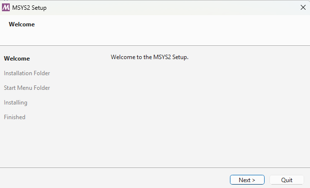
Download and run the installer :

Welcome to the MSYS2 Setup 

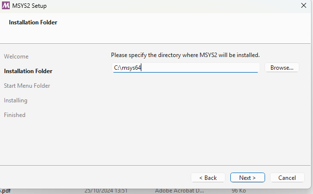
Choose the installation folder :

Installation folder


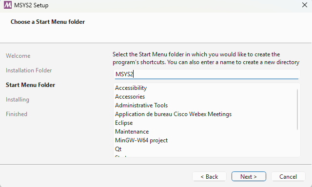
Follow installation steps : 

Installation steps

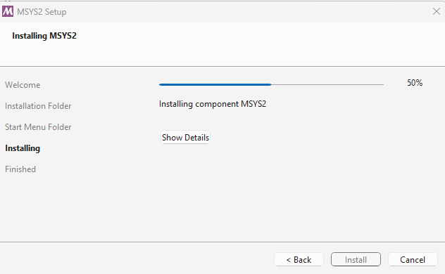
Wait for installation process to finish : 

Wait...


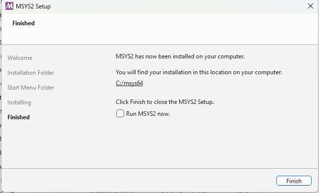
then click on Finish : 

Finish

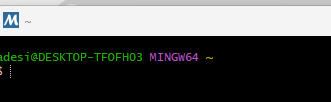
Once installed, the MinGW64 bash can be launched from Windows menu :

Windows menu

MinGW64


Step 2. Install compiler tools and dependencies

Msys provides the package manager , called pacman, that can be used to install all necessary tools and dependencies Doc here : https://www.msys2.org/docs/package-management/

You will need to install the following packages ( you can use the commands below provided for each of them, or look for in https://packages.msys2.org/queue and choose Mingw64 binaries) : 

  • GCC: pacman -S mingw-w64-x86_64-gcc

  • CMake: pacman -S mingw-w64-x86_64-ccmake

  • Make: pacman -S mingw-w64-x86_64-make

  • Boost: pacman -S mingw-w64-x86_64-boost

  • Dlfcn: pacman -S mingw-w64-x86_64-dlfcn

  • Spdlog: pacman -S mingw-w64-x86_64-spdlog

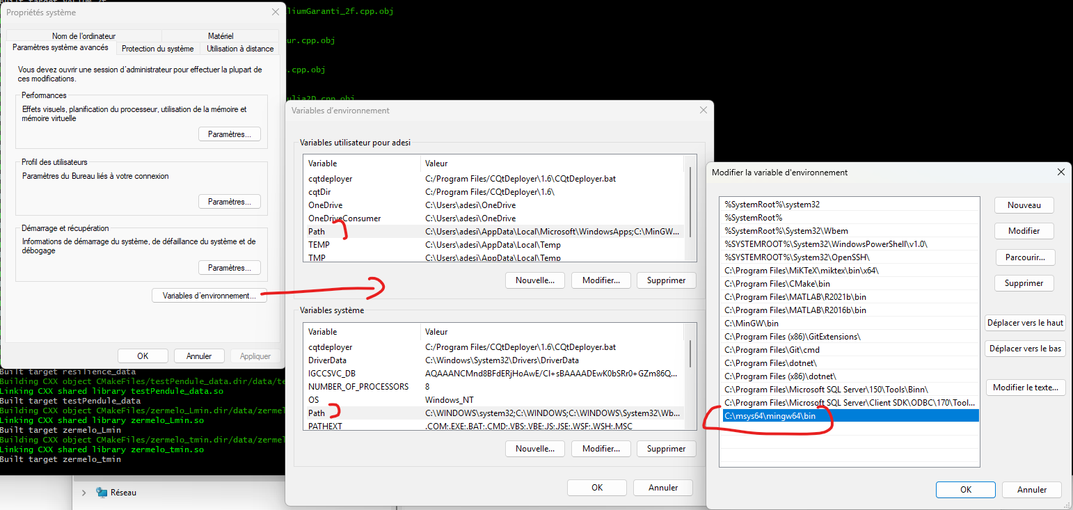
To finish the installation, add into System Path variable the path to Mingw64 binaries C:\msys64\mingw64\bin:

Add path variable


After this operation you may need to restart your computer to ensure that the Path modifications are well registered. 


Step 3. Copy VIABLAB in MSyS folder 

Go to https://github.com/lastre-viab/VIABLAB, click on Code button and download the ZIP file VIABLAB-main.zip. 

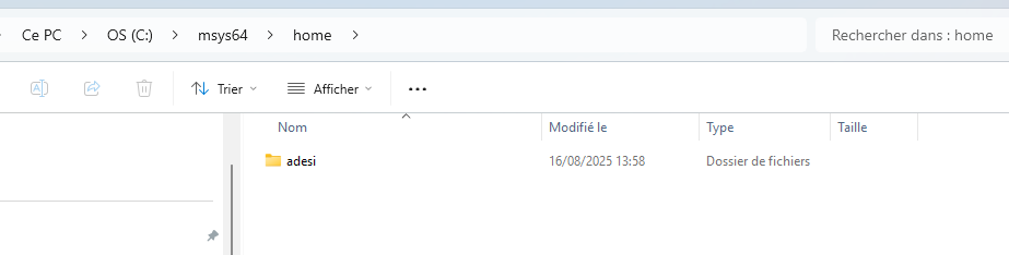
By default the MSyS shell is open in /home/username folder. You can see it in FileExplorer 


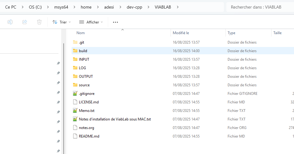
Open this folder in FileExplorer, create the folder dev-cpp that will contain the  program and results and unzip VIABLAB-main.zip there. Example : 


Step 4. Install Eclipse (Integrated development environment) (optional)

Go to  https://www.eclipse.org/downloads/packages/release/kepler/sr2/eclipse-ide-cc-developers

Click on "download", again "download".

Once downloaded, run the installer and choose  Eclipse IDE for C/C++ developers.

Click on ‘’launch’’, and 'launch" again.

Step 5. Build VIABLAB in MSyS folder 

Go back to the MSyS MINGW64 shell . You are now ready to build VIABLAB code. 

First, go to the build folder (create it if it doesn't exist) of VIABLAB in bash (depending on your personal installation). With the example folder shown above : 

cd dev-cpp/VIABLAB-main/build/

Then cmake command : 

  • cmake -G"MinGW Makefiles" -D BUILD_LIB=OFF ../source

  • If you use Eclipse C++ IDE, you can use the cmake command below to generate Eclipse project settings and enable debugging in Eclipse :

    cmake -G"Eclipse CDT4 - MinGW Makefiles" -D CMAKE_BUILD_TYPE=Debug -D BUILD_LIB=OFF ../source

    After running CMake, the project is ready to be imported into Eclipse: the build directory (initially empty) contains the data generated by CMake.

    In Eclipse, go to the File menu => Import and select the Existing Projects into Workspace option.

    Click Next.

    Then, in the following window, select the build directory.

    Click Finish.

    After the import, you will see the project tree in the left panel.

Note that cmake command must be executed only once, on first installation; further, only the make command below will be sufficient to build the code : 

mingw32-make

Once the compilation process finished, the executable viabLab.exe is created in build folder. 


Théorie mathématique de la viabilité en anglais

Université des Antilles, Pôle Martinique
01-08-2025
20
Niveau de difficulté
Présentation de l'atelier

Cet atelier propose une introduction appliquée à la théorie de la viabilité, notamment dans le cadre des écosystèmes soumis à des contraintes environnementales. Les participants exploreront comment formaliser des politiques durables de gestion à l’aide d’algorithmes de viabilité, et comment modéliser la résilience d’un système via des cas concrets comme l’eutrophisation d’un lac ou la gestion d'une population.

Objectifs de l'atelier
  • Comprendre les bases mathématiques de la viabilité dynamique.
  • Utiliser des modèles simples pour représenter des contraintes écologiques.
  • Manipuler un simulateur interactif pour visualiser les trajectoires viables.
  • Favoriser les échanges entre chercheurs, étudiants et praticiens.
Programme

LUNDI 27 AVRIL

8h15 - Rendez-vous de l’ensemble des participants devant la Bibliothèque Universitaire


SESSION 1 : POSER UN PROBLEME EN VIABILITE

Animateur : Bates – De Lapparent - Lavallée - Désilles

8h30 - 8h50 La viabilité mathématique en question ? (Samuel Bates)

8h50 - 9h50 Concept et illustration du noyau de viabilité (François Lavallée)

Pause & discussion

10h00-11h15 Formuler mathématiquement un problème de viabilité (François Lavallée)

11h15-12h00 Cas de résolution analytique de la viabilité (François Lavallée)

Déjeuner

13h30-14h15 Cas de résolution numérique de la viabilité (François Lavallée)

14h15-15h00 Cas de résolution de viabilité avec cible terminale (François Lavallée)

Pause & discussion

15h15-16h00 Cas de résolution de viabilité en situation de risque (François Lavallée)

16h00-16h45 Cas de résolution de viabilité en situation d’incertitude (François Lavallée)

Pause & discussion

17h00-17h45 Cas de résolution de viabilité multi-agent (Alice De Lapparent)


MARDI 28 AVRIL

SESSION 2 : L’INFORMATIQUE DE LA VIABILITE

Animateur : Désilles - Lavallée


8h00-9h00 Préparation à l’informatique de la viabilité (Anya Désilles)

9h00-10h30 Présentation du logiciel Viablab (Anya Désilles)

Pause & discussion

10h45-11h15 Enjeux informatiques sur les noyaux de viabilité (Anya Désilles)

11h15-12h00 Enjeux informatiques sur les trajectoires de viabilité (Anya Désilles)

Déjeuner

13h30-15h30 Atelier de manipulation du Logiciel autour d’un cas d’étude (1/2) (François Lavallée & Anya Désilles)

Pause & discussion

15h45-17h45 Atelier de manipulation du Logiciel autour d’un cas d’étude (2/2) (François Lavallée & Anya Désilles)


MERCREDI 29 AVRIL

SESSION 3 : ATELIERS THEMATIQUES D’APPLICATION

Animateurs Désilles - Gloglo


8h00-10h00 Atelier autour de AgroViablab : Illustration vers une montée en
complexité (Anya Désilles)

Pause & discussion

10h15-12h15 Brainstorming autour d’AgroViablab (collectif)

Déjeuner

13h45-15h45 Atelier d’application sur un système monétaire : Illustration vers une simplification de complexité (Beringer Gloglo)

15h45-17h45 Brainstorming sur les applications (collectif)


18h00-19h00 Séminaire sur la viabilité en économie monétaire (en marge de l’école chercheur à destination des étudiants de Master d’économie) (Beringer Gloglo, Samuel Bates)


JEUDI 30 AVRIL


SESSION 4 : MODELISATION EN VIABILITE

8h00-09h00 Brainstroming autour d’un 1er sujet de modélisation (collectif)

9h00-10h00 Brainstroming autour d’un 2e sujet de modélisation (collectif)

Pause & discussion

10h15-11h15 Brainstroming autour d’un 3e sujet de modélisation (collectif)

11h15-12h00 Retour d’expériences


Déjeuner & clôture hors les murs (13h00-17h00 : Saint-Pierre)

Description localisation

L'atelier aura lieu à l'Université des Antilles, Pôle Martinique

Liste des participants
Science économique

- Pablo Andres-Domenech
- Valérie Angeon
- Samuel Bates
- Abdoul Cisse
- Issaka Dialga
- Beringer Gloglo
- Thaly Janloup
- Eric Kamwa
- Kevin Spinassou

Mathématique

- Severine Andouze/Bernard
- James Larrouy
- François Lavallée
- Loïc Louison
- Paul Silvere Nuiro

Géographie

- Etienne Delay
- Pastel Audrey

Agronomie

- Alice De-Lapparent

Informatique

- Anya Désilles

[Texte] Installation ViabLab with Gui v3.0

Niveau de difficulté
Thématique
Présentation formation

Sous MAC

Pas possible pour le moment, le fichier binaire n'est disponible que pour Linux et Windows, il faut cloner à partir d'un dépôt.


Sous LINUX

Prérequis : 

  • Avoir installé g++ :   

 Pour vérifier si g++ est installé, dans un terminal : 

g++ --version

Si g++ n'est pas encore installé sur votre système :        

sudo apt install g++
  • Avoir installé cmake version 3.22.1 : 

Pour vérifier si cmake est installé et connaitre sa version, dans un terminal :

cmake --version

Si ce n'est pas la bonne version , supprimer les versions existantes de CMake, dans un terminal :

sudo apt remove --purge cmake

Vérifier la version de votre Ubuntu, dans un terminal : 

lsb_release -a

 Si votre version est 22.04, installer CMake 3.22.1 automatiquement :

    sudo apt update
    sudo apt install cmake

Si votre version n’est pas 22.04, installer les dépendances nécessaires :
 

    sudo apt update
    sudo apt install -y build-essential libssl-dev

 Télécharger CMake 3.22.1 :

       wget https://github.com/Kitware/CMake/releases/download/v3.22.1/cmake-3.22.1.tar.gz

  Extraire l'archive :

    tar -zxvf cmake-3.22.1.tar.gz
    cd cmake-3.22.1

    Construire et installer :

    ./bootstrap
    make -j$(nproc)      # Compiles using all available CPU cores
    sudo make install

Vérifier la version de cmake, dans un terminal :

cmake --version

Doit afficher  cmake version 3.22.1.

  • Avoir installé l'IDE Eclipse (facultatif)

    sudo apt-get install -y eclipse-cdt


Installation de Viablab :

chmod +x InstallerViabLabGui_v1_linux.run
  • Pour exécuter l'installeur
./InstallerViabLabGui_v1_linux.run
  • Next - Next - Next - Install - Finish
  • Puis se placer à l’aide de la commande cd dans le répertoire build : ~/ViabLabGui/bin/VIABLAB/build  
  • puis, pour une utilisation sans l'IDE Eclipse :
cmake -G "Unix Makefiles" ../source
make

 L'exécutable viabLabExe apparaît dans le répertoire build ! 

  • ou, pour une utilisation avec Eclipse :
cmake -D_ECLIPSE_VERSION=4.5 -DCMAKE_BUILD_TYPE=Debug ../source -G"Eclipse CDT4 - Unix Makefiles" -DCMAKE_ECLIPSE_GENERATE_SOURCE_PROJECT=TRUE


Sous WINDOWS :

Prérequis : 

  • Avoir installé MinGW, une distribution de compilateurs C/C++ GNU pour Windows :   

 A l'adresse https://sourceforge.net/projects/mingw/files/latest/download , téléchargez l'application MinGW Installation Manager.

Ouvrir cette application 

Dans le panneau gauche, développer All packages => MinGW, sélectionner MinGW Base System. Sélectionner dans la liste des packages tous les packages dont le nom contient « pthread », choisir Mark For Installation. Faire de même pour les packages gcc, omp, g++, libstd, mingw s’ils ne sont pas sélectionnés.

Une fois les packages sélectionnés, dans le menu Installation, cliquer sur Apply changes et attendre la fin d’installation.

Ajouter l’emplacement de l’installation MinGW dans la variable PATh du système :

Dans paramètres/settings du système, on cherche environmental/environnement et on clique dans «edit environment variables for your account »

Aller dans Path, edit, new et on copie colle : C:\MinGW\bin

Eteindre et redémarrer l'ordinateur.
 

  • Avoir installé cmake version 3.31.7:

Pour vérifier si cmake est installé et connaitre sa version, dans un terminal :

??

Si ce n'est pas la bonne version , supprimer les versions existantes de CMake, dans un terminal :

??

 Aller à l'adresse https://github.com/Kitware/CMake/releases/download/v3.31.7/cmake-3.31.7-windows-x86_64.msi pour télécharger le Windows x64 installer.

Vérifier la version de cmake, dans un terminal :

????

Doit afficher  cmake version 3.31.7.

  • Avoir installé Eclipse Environnement de développement intégré) (facultatif) :  

Aller à l'adresse  https://www.eclipse.org/downloads/packages/release/kepler/sr2/eclipse-ide-cc-developers

Cliquer sur download, à nouveau sur download.

Une fois téléchargé, cliquer sur l’installeur et chosir  Eclipse IDE for C/C++ developers

On ‘’launch’’ par la suite (première exécution pour voir que tout fonctionne)

On ‘’launch’’ de nouveau.


Installation de Viablab :

??
  • Pour exécuter l'installeur
??
  • Next - Next - Next - Install - Finish
  • Puis ouvrir un PowerShell, se placer à l’aide de la commande cd dans le répertoire build : ~/ViabLabGui/bin/VIABLAB/build  
  • puis, pour une utilisation sans l'IDE Eclipse :
cmake -G "MinGW Makefiles" ../source
make

 L'exécutable viabLabExe apparaît dans le répertoire build

  • ou, pour une utilisation avec Eclipse :
cmake -G"Eclipse CDT4 - MinGW Makefiles" -D CMAKE_BUILD_TYPE=Debug ../source

Après l’exécution de cmake le projet est prêt pour être importé dans Eclipse : le répertoire build ( vide au début) contient les données générées par cmake.

Dans Eclipse, aller dans le menu File => Import et sélectionner l’option Existing Projects into Workspace

Cliquer sur Next

Ensuite dans le fenêtre suivante sélectionner le répertoire build

Cliquer sur Finish

Après l’import on voit l’arborescence du projet dans le panneau gauche